Malte Laustsen1,2,3, Mads Andersen4, Rong Xue3,5,6, Kristoffer H. Madsen2,7, and Lars G. Hanson1,2
1Section for Magnetic Resonance, DTU Health Tech, Technical University of Denmark, Kgs. Lyngby, Denmark, 2Danish Research Centre for Magnetic Resonance, Centre for Functional and Diagnostic Imaging and Research, Copenhagen University Hospital Hvidovre, Hvidovre, Denmark, 3Sino-Danish Center, University of Chinese Academy of Sciences, Beijing, China, 4Philips Healthcare, Copenhagen, Denmark, 5State Key Laboratory of Brain and Cognitive Science, Beijing MR Center for Brain Research, Institute of Biophysics, Chinese Academy of Sciences, Beijing, China, 6Beijing Institute for Brain Disorders, Beijing, China, 7DTU Compute, Technical University of Denmark, Kgs. Lyngby, Denmark
1Section for Magnetic Resonance, DTU Health Tech, Technical University of Denmark, Kgs. Lyngby, Denmark, 2Danish Research Centre for Magnetic Resonance, Centre for Functional and Diagnostic Imaging and Research, Copenhagen University Hospital Hvidovre, Hvidovre, Denmark, 3Sino-Danish Center, University of Chinese Academy of Sciences, Beijing, China, 4Philips Healthcare, Copenhagen, Denmark, 5State Key Laboratory of Brain and Cognitive Science, Beijing MR Center for Brain Research, Institute of Biophysics, Chinese Academy of Sciences, Beijing, China, 6Beijing Institute for Brain Disorders, Beijing, China, 7DTU Compute, Technical University of Denmark, Kgs. Lyngby, Denmark
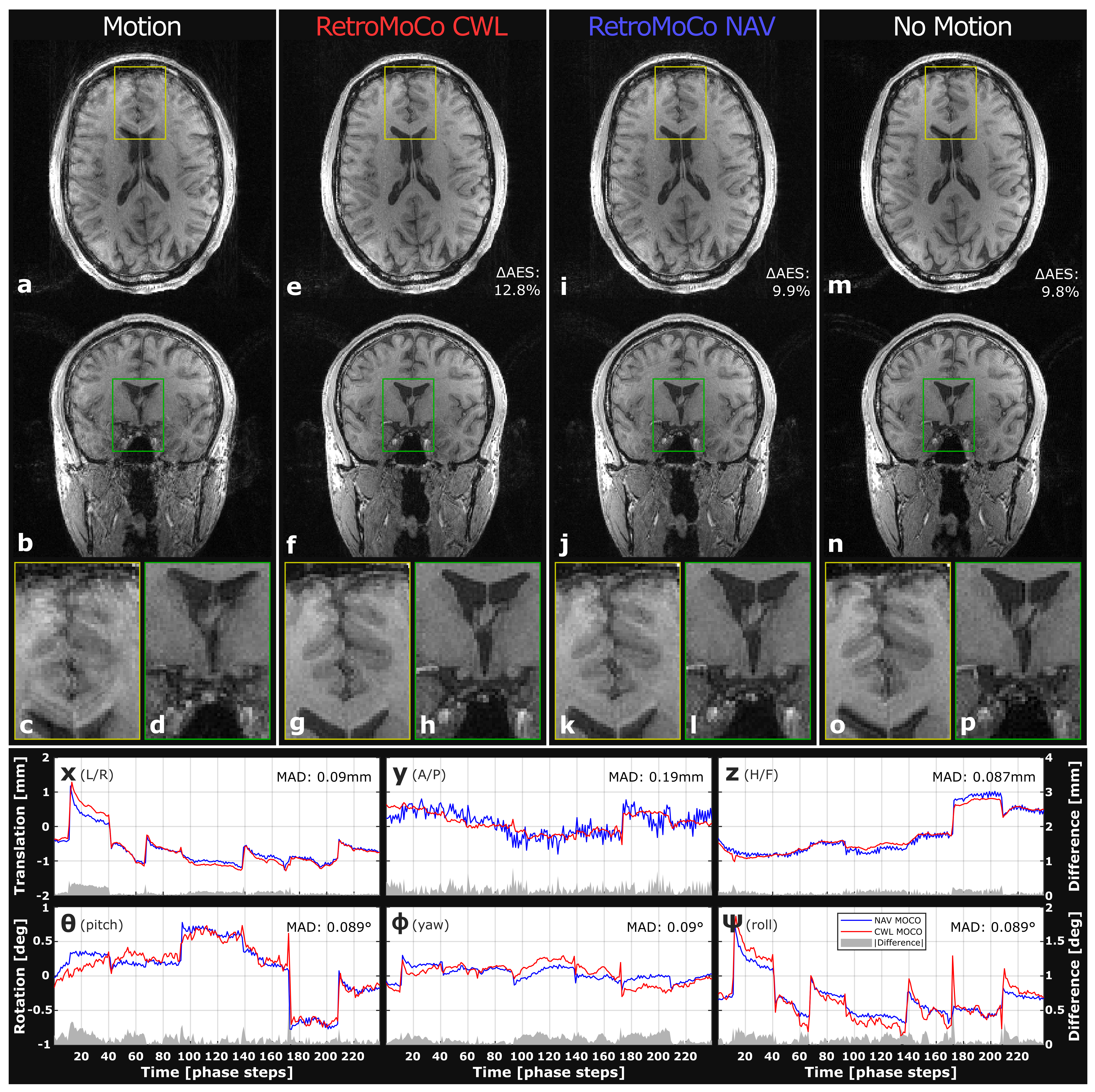
Motion tracking based on carbon wire loops show close similarity to interleaved navigators (MAD: [0.13,0.33,0.12]mm, [0.28,0.15,0.22]deg)
yielding similar improvement to image sharpness (ΔAES: 12%) after
retrospective correction of T1w 3D images, without sequence modification.
Figure
3: Retrospective
motion correction of a structural scan with instructed movement (Table 1: subject 2, trial 4) with moderate motion of 1-2mm (x,y,z) and 1-2deg (θ,ϕ,ψ).
Tracking curves for CWLs and NAVs (red, blue respectively) show high degree of similarity (low mean absolute difference,
MAD), with largest discrepancy (gray) in y-translations. A substantial
increase to visual sharpness (e-l) is evident after retrospective correction
using either tracking method. Both methods lead to an increase to average
edge strength (AES) of 12.8/9.9% for CWLs and NAVs, respectively.
Figure
1:
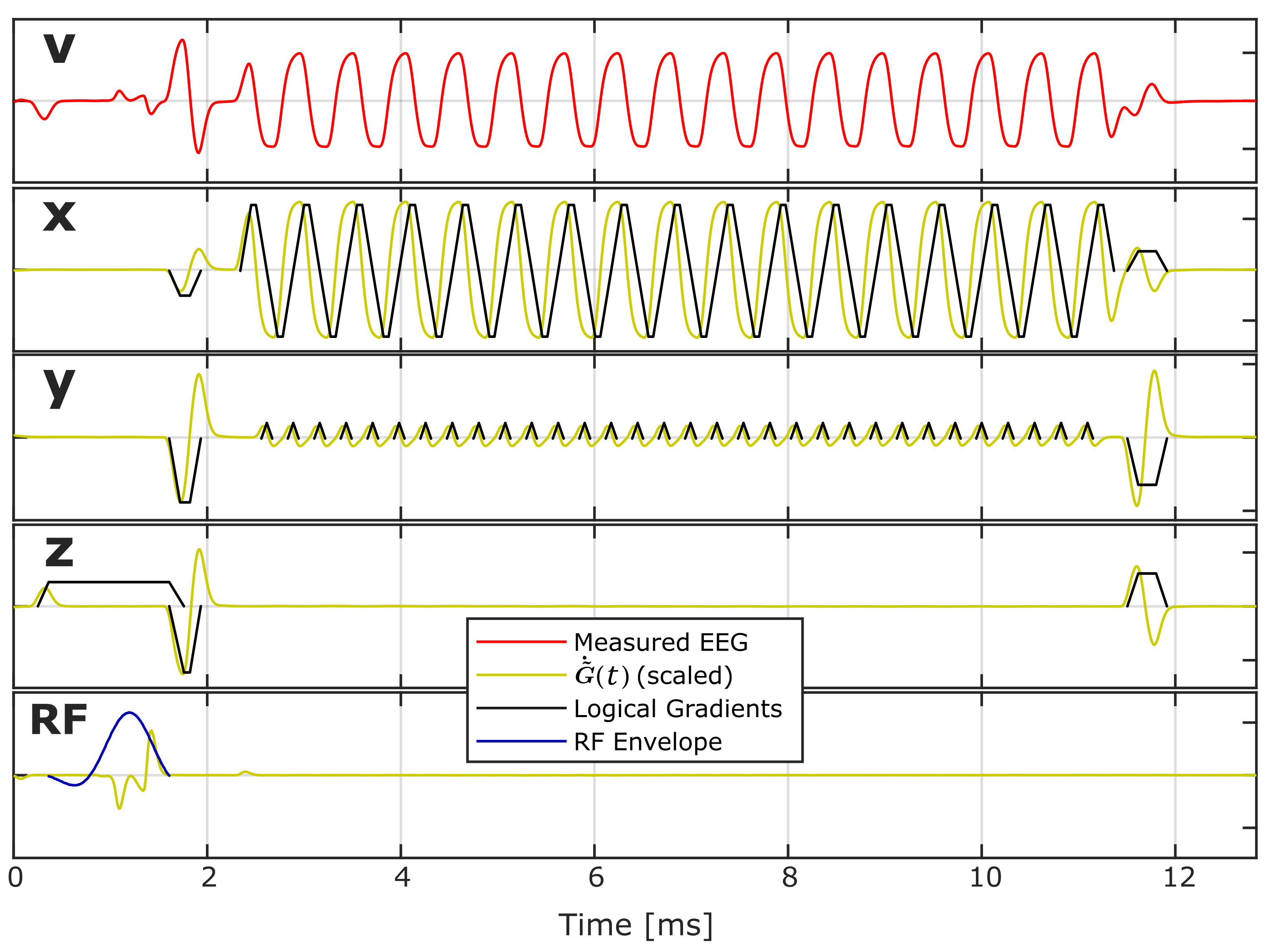
Measured wire loop signal $$$\mathit{v}_i(t)$$$ for part of a navigator consisting of a weighted sum of columns of $$$\dot{\tilde{\pmb{\mathit{G}}}}(t)$$$, which resemble filtered time derivatives of gradient
activity, and are found by sampling the sequence in a static phantom
pre-scan with only one active gradient component $$$\mathit{g}_x(t)$$$, $$$\mathit{g}_y(t)$$$,
$$$\mathit{g}_z(t)$$$, or active RF. Each wire loop ($$$i=[1,2,\ldots ,I]$$$) measures a unique weighted sum dependent
on loop position, orientation, and geometry.