Ke Wang1, Michael Kellman2, Christopher M. Sandino3, Kevin Zhang1, Shreyas S. Vasanawala4, Jonathan I. Tamir5, Stella X. Yu6, and Michael Lustig1
1Electrical Engineering and Computer Sciences, University of California, Berkeley, Berkeley, CA, United States, 2Pharmaceutical Chemistry, University of California, San Francisco, Berkeley, CA, United States, 3Electrical Engineering, Stanford University, Stanford, CA, United States, 4Radiology, Stanford University, Stanford, CA, United States, 5Electrical and Computer Engineering, The University of Texas at Austin, Austin, TX, United States, 6International Computer Science Institute, University of California, Berkeley, Berkeley, CA, United States
1Electrical Engineering and Computer Sciences, University of California, Berkeley, Berkeley, CA, United States, 2Pharmaceutical Chemistry, University of California, San Francisco, Berkeley, CA, United States, 3Electrical Engineering, Stanford University, Stanford, CA, United States, 4Radiology, Stanford University, Stanford, CA, United States, 5Electrical and Computer Engineering, The University of Texas at Austin, Austin, TX, United States, 6International Computer Science Institute, University of California, Berkeley, Berkeley, CA, United States
We present a memory-efficient learning (MEL) framework for high-dimensional MR reconstruction to enable training larger and deeper unrolled networks on a single GPU. We demonstrate improved image quality with learned reconstruction enabled by MEL for 3D MRI and 2D cardiac cine applications.
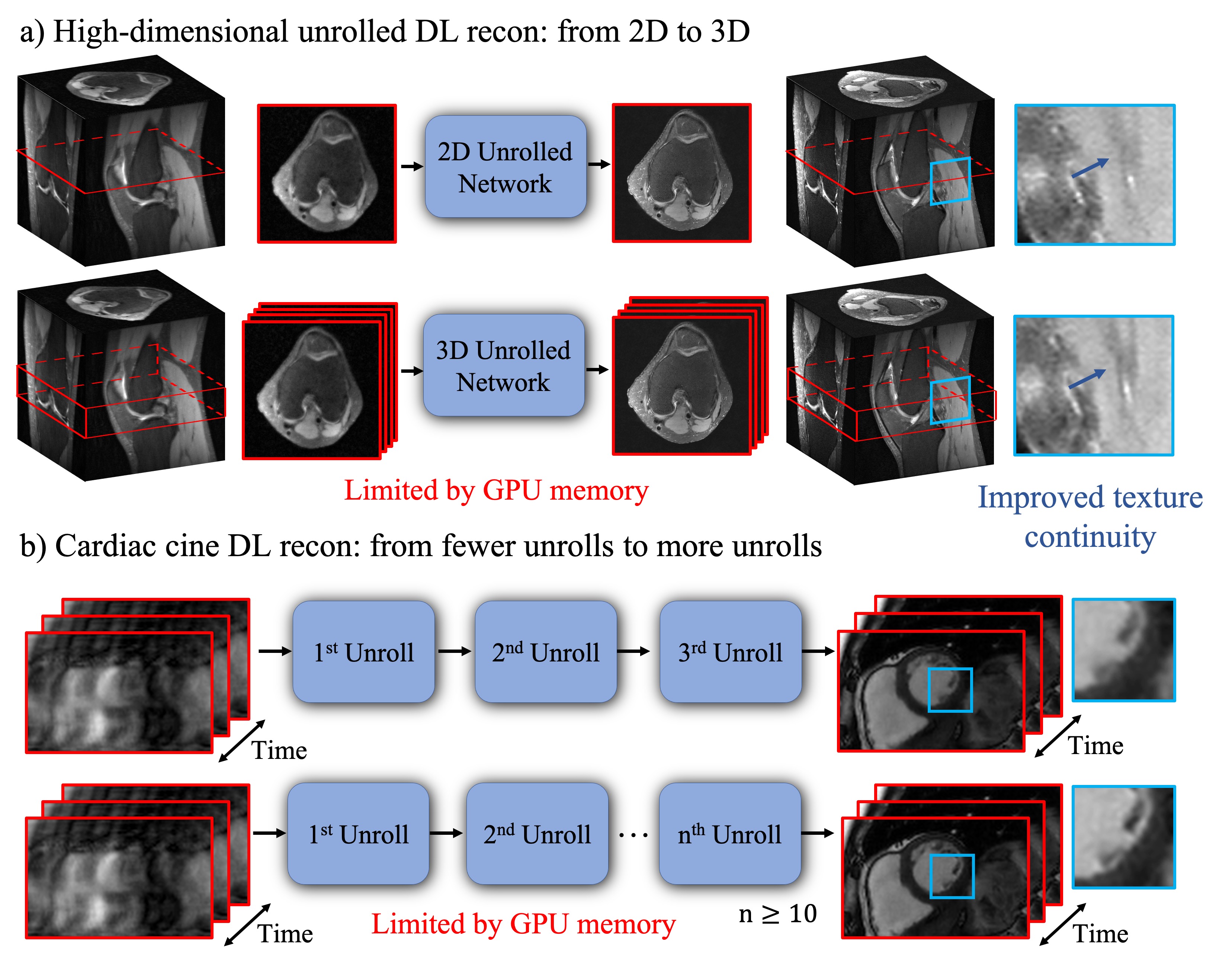
Figure 1. GPU memory limitations for high-dimensional unrolled DL recons: a) Conventionally, in order to reconstruct a 3D volume, each slice in the readout dimension is independently passed through a 2D unrolled network and then re-joined into a 3D volume. In contrast, 3D unrolled networks require more memory but use 3D slabs during the training, which leverages more data redundancy. b) Typically, cardiac cine DL recons are often performed with a small number of unrolls due to memory limitations. More unrolls are able to better learn the finer spatial and temporal textures.
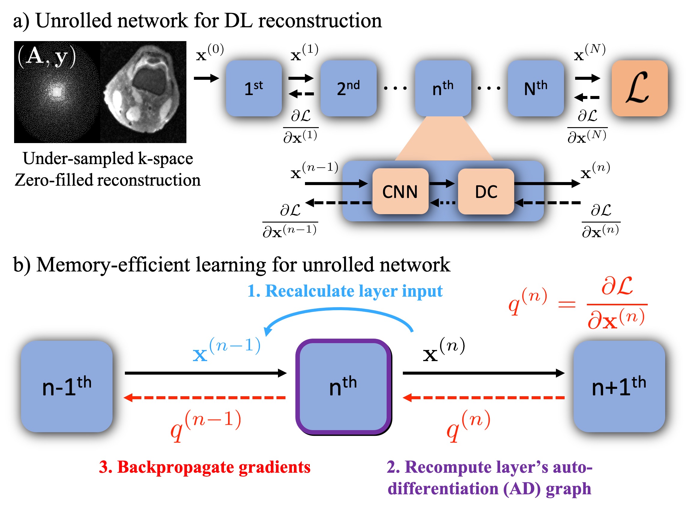
Figure 2. a) Unrolled networks are formed by unrolling the iterations of an image reconstruction optimization. Each unroll consists of a CNN-based regularization layer and a DC layer. Conventionally, gradients of all layers are computed simultaneously, which requires a significant GPU memory cost. b) Memory-efficient learning procedure for a single layer: 1) Recalculate the layer’s input $$$\mathbf{x}^{(n-1)}$$$, from the known output $$$\mathbf{x}^{(n)}$$$. 2) Reform the AD graph for that layer. 3) Backpropagate gradients $$$q^{(n)}$$$ through the layer’s AD graph.