Avery JL Berman1,2, Avery JL Berman1,2, Fuyixue Wang1,3, Kawin Setsompop4,5, J. Jean Chen6,7, and Jonathan R Polimeni1,2,3
1Athinoula A. Martinos Center for Biomedical Imaging, Massachusetts General Hospital, Charlestown, MA, United States, 2Department of Radiology, Harvard Medical School, Boston, MA, United States, 3Harvard-MIT Division of Health Sciences and Technology, Massachusetts Institute of Technology, Cambridge, MA, United States, 4Department of Radiology, Stanford University, Palo Alto, CA, United States, 5Department of Electrical Engineering, Stanford University, Palo Alto, CA, United States, 6Rotman Research Institute, Baycrest Health Sciences, Toronto, ON, Canada, 7Department of Medical Biophysics, University of Toronto, Toronto, ON, Canada
1Athinoula A. Martinos Center for Biomedical Imaging, Massachusetts General Hospital, Charlestown, MA, United States, 2Department of Radiology, Harvard Medical School, Boston, MA, United States, 3Harvard-MIT Division of Health Sciences and Technology, Massachusetts Institute of Technology, Cambridge, MA, United States, 4Department of Radiology, Stanford University, Palo Alto, CA, United States, 5Department of Electrical Engineering, Stanford University, Palo Alto, CA, United States, 6Rotman Research Institute, Baycrest Health Sciences, Toronto, ON, Canada, 7Department of Medical Biophysics, University of Toronto, Toronto, ON, Canada
We introduced BOLD signal simulations that incorporate image encoding gradients. We examined large-vessel Spin-Echo BOLD contamination as a function of EPI readout duration, vessel size, voxel size, and cortical depth, and reproduced experimental results related to the readout duration.
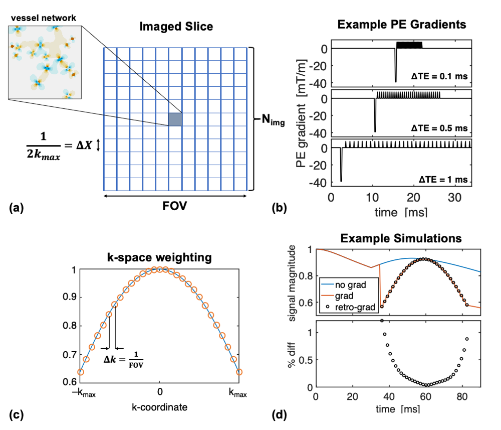
Fig 1: Schematic of the image-encoding framework. (a) Overview of the "imaged" slice, consisting of the simulated vessel network at its center and surrounded by zero magnetization, effectively a Kronecker delta-function. (b) Example EPI PE gradient train at multiple echo-spacings. (c) The sinc-weighting imposed by the encoding gradients. (d) Example SE simulations without imaging gradients (blue), with imaging gradients (orange), and with the k-space weighting retrospectively applied to the non-encoded simulation (black circles). The difference is up to a maximum of ~1%.
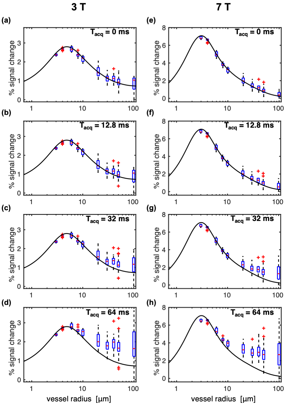
Fig. 3: Box plots of SE-BOLD percent signal change vs. vessel radius for multiple acquisition window durations (Tacq), and where the voxel size was held constant, resulting in decreasing numbers of vessels for the larger radii. Simulations were performed at 3T (left) and 7T (right) with Tacq increasing from 0 (a,e) to 64 ms (d,h). For comparison, the black curves are the spline fits to the SE data with Tacq = 0 ms in Fig. 2. Phase-encoding gradients were incorporated retrospectively as described by Eq. (2) in the Methods. Note the different scales for 3T and 7T.