Jeremiah Sanders1, Henry Mok2, Alexander Hanania3, Aradhana Venkatesan4, Chad Tang2, Teresa Bruno2, Howard Thames5, Rajat Kudchadker6, and Steven Frank2
1Imaging Physics, UT MD Anderson Cancer Center, Houston, TX, United States, 2Radiation Oncology, UT MD Anderson Cancer Center, Houston, TX, United States, 3Radiation Oncology, Baylor College of Medicine, Houston, TX, United States, 4Diagnostic Radiology, UT MD Anderson Cancer Center, Houston, TX, United States, 5Biostatistics, UT MD Anderson Cancer Center, Houston, TX, United States, 6Radiation Physics, UT MD Anderson Cancer Center, Houston, TX, United States
1Imaging Physics, UT MD Anderson Cancer Center, Houston, TX, United States, 2Radiation Oncology, UT MD Anderson Cancer Center, Houston, TX, United States, 3Radiation Oncology, Baylor College of Medicine, Houston, TX, United States, 4Diagnostic Radiology, UT MD Anderson Cancer Center, Houston, TX, United States, 5Biostatistics, UT MD Anderson Cancer Center, Houston, TX, United States, 6Radiation Physics, UT MD Anderson Cancer Center, Houston, TX, United States
Spatial entropy clusters with the highest entropy were
located around the circumference of the prostate, especially at
junctions between the target and surrounding OARs (bladder neck, prostate-SV junction, region along prostate and rectal wall,
prostate apex-EUS junction).

Figure 2. Spatial entropy maps for human and computer observer populations in 8 example patients. Spatial entropy maps were computed by first grouping the predictions from DL models trained with the same loss function. Four loss functions were investigated including crossentropy, DSC, Jaccard, and focal.
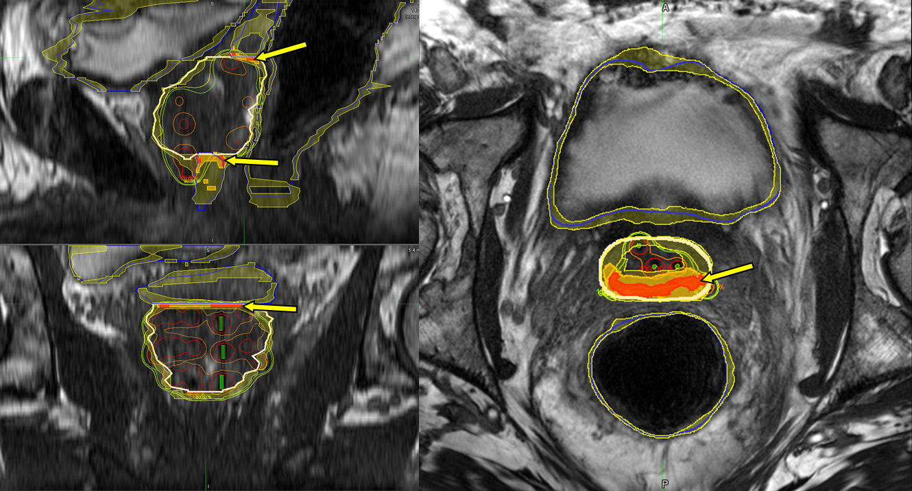
Figure 3. Autocontouring predictions (prostate: thick white line, OARs: blue lines)
displayed with spatial entropy maps (transparent regions; yellow–30% of max entropy,
orange-70% of max entropy, red-90% of max entropy) overlaid on post-implant prostate MRIs
in a commercial treatment planning system. Arrows indicate regions of high
spatial entropy clusters at organ junctions where physicians can review and
potentially refine the automated predictions.