-
In-vivo B0 shimming of the liver using a local array of shim coils in combination with 2nd order spherical harmonics at 7T
Lieke van den Wildenberg1, Quincy van Houtum1, Wybe van der Kemp1, Catalina Arteaga de Castro1, Alex Bhogal1, Paul Chang2, Sahar Nassirpour2, and Dennis Klomp1
1Radiology Department, UMC Utrecht, Utrecht, Netherlands, 2MR Shim GmbH, Reutlingen, Germany
The B0 field inhomogeneity in the liver at 7T can be
reduced using a local shim coil array combined with 2nd order
spherical harmonics B0 shimming correction methods which can
potentially lead to an inhomogeneity reduction of 44%.
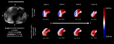
Figure
5: In-vivo B0 field mapping of
the liver in a healthy volunteer during free breathing with two different B0
shimming methods: 1) scanner shim (2nd order) and 2) array of shim
coils in combination with the conventional second scanner shim. A: anterior, P: posterior, R: right, L:
left, H: head, F: feet, and std: standard deviation.
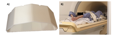
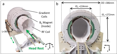
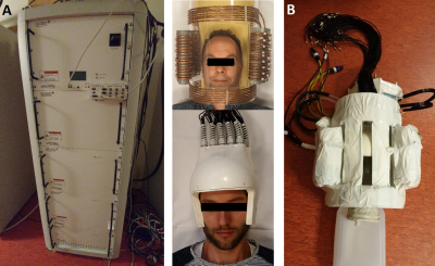
Figure
1: A) The
array of shim coils B) used around the body array in the 7T MR system
-
“RF transparent” local B0 shim coil
Xinqiang Yan1,2
1Vanderbilt University Institute of Imaging Science, Nashville, TN, United States, 2Department of Radiology and Radilogical Science, Vanderbilt University Medical Center, Nashville, TN, United States
“RF transparent” local B0 shim coil have minimal crosstalk
with RF coils without using massive bulky RF chokes.
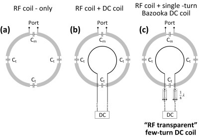
Figure
1 Circuit diagrams of RF-only
coil, RF coil + DC coil, and RF coil + “RF transparent” DC coil. Note that in practice, feed wires of DC coils are typically twisted to cancel the
Lorentz force. For simplicity, straight feed wires were shown here. For Bazooka-feedline [5] few-turn “RF transparent” DC coil, the shield of twisted wires (could be one
shield for each wire or one shield for both wires) was shorted at the position
that is 1/4 wavelength away from the DC coil, forming open circuits and block
RF signal going through.
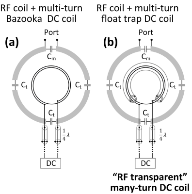
Figure
2 Circuit diagrams of many-turn
“RF transparent” DC coil using float trap design. For many-turn DC coil, it
may resonate close to the RF frequency even the feed port is broken using
the bazooka feedline method (A). In this case, it still can be seen as a
coupled lossy resonator and leads to SNR loss.
The float trap [6] is a concentric resonator that inductively couples and traps
the RF signal going through it. It is expected to break every turn of the DC coil that goes
through the trap and thus avoid unwanted resonate modes.
-
Shim Coils Tailored for Correction of B0 Inhomogeneity in the Human Brain (SCOTCH) at Ultra High Field
Bruno Pinho-Meneses1, Jason Stockmann2,3, Edouard Chazel1, Paul-François Gapais1, Eric Giacomini1, Franck Mauconduit1, Alexandre Vignaud1, Michel Luong4, and Alexis Amadon1
1Université Paris-Saclay, CEA, CNRS, BAOBAB, NeuroSpin, Gif-sur-Yvette, France, 2Athinoula A. Martinos Center for Biomedical Imaging, Charlestown, MA, United States, 3Harvard Medical School, Boston, MA, United States, 4Université Paris-Saclay, CEA, Institut de Recherche sur les Lois Fondamentales de l'Univers, Gif-sur-Yvette, France
A 2-layer 36-channel optimized Multi-Coil Array for B0 shimming of the human brain was designed. A prototype was built and in-vivo GRE and EPI acquisitions were performed, confirming high inhomogeneity reduction and artifact mitigation after shimming with the optimized MCA.
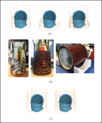
Figure 1: a) From left to right: Ideal
channel disposition and geometry for first and second layers, both layers resulting from the
SVD-based MCA optimization; and ideal 2-layer 36-channel system. b) The two
prototype layers and the assembled shimming system with RF housing in the
interior of the shim layers. c) Simulation models of generic 24-ch (left) and 48-ch (right) M-MCA used for comparison. Circular coil radii are 4.5-cm and 3.5-cm,
respectively.
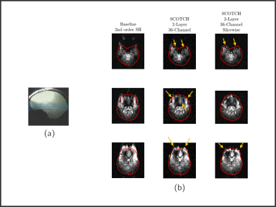
Figure 5: a) Brain mask overlay (green)
considered for optimal current calculations for global shimming and selected
slices (blue) presented in b) rs-EPI acquisitions. Baseline, global and
slicewise (dynamic) 2-layer 36-channel SCOTCH shimming are shown. Gradient Echo rS-EPI sequence
parameters were 2-mm in-plane resolution, fifteen 3-mm-thick slices,
TE/TR=44/84000ms. Yellow arrows highlighting zones with significant
improvement.
-
Designing a high-density combined RF/B0 shim coil for imaging the brain at 7T
Paul Chang1, Sahar Nassirpour1, Kaizad Rustomji2, Elodie Georget2, Ingmar Voogt3, Aidin Haghnejad3, Evita Wiegers4, Jannie Wijnen4, and Dennis Klomp4
1MR Shim GmbH, Reutlingen, Germany, 2Multiwave Imaging, Marseille, France, 3WaveTronica, Utrecht, Netherlands, 4UMC Utrecht, Utrecht, Netherlands
To minimize RF interference, the Rx loops should be larger than shim coils with an optimal gap of 4cm. An optimized distribution of the shim loops tailored to the brain anatomy achieved significant B0 shimming improvement (43% compared to 2nd order) with at max 1.2dB loss in MR sensitivity.
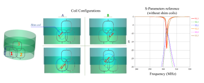
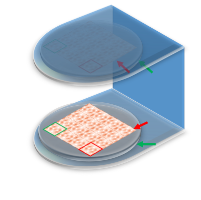
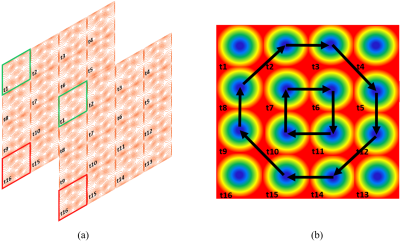
Figure 1 Three RF loops (84mm diameter each) were arranged in the configuration shown on the left. The four different settings for the shim coildiameter/positioning used in the numerical simulation are also shown. The reference S-parameter curves (in the absence of the shim coils) are shown on theright.
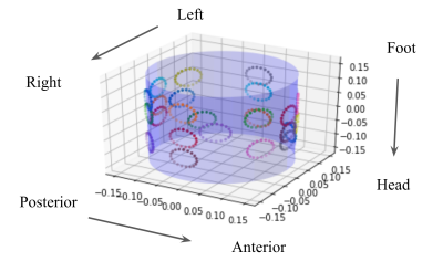
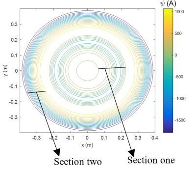
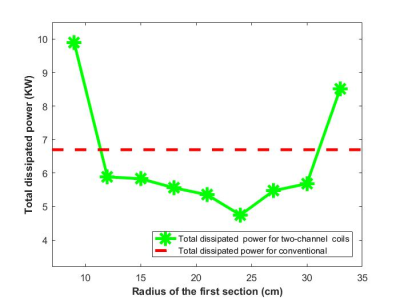
Figure 4 Optimal arrangement of 24 shim coils on a cylindrical holder (units in [m]).
-
Shielded coaxial cable coils for transmit, receive and B0 shimming in a 7T neck array
Vincent O. Boer1, Jan Ole Pedersen2, Hørður Andreasen3, Sadri Güler1,4, Vitaliy Zhurbenko3, Jason Stockmann5, Irena Zivkovic6, and Esben Thade Petersen1,4
1Danish Research Centre for Magnetic Resonance, Centre for Functional and Diagnostic Imaging and Research, Copenhagen University Hospital, Hvidovre, Denmark, 2Philips Healthcare, Copenhagen, Denmark, 3Department of Electrical Engineering, Technical University of Denmark, Kongens Lyngby, Denmark, 4Section for Magnetic Resonance, DTU Health Tech, Technical University of Denmark, Kongens Lyngby, Denmark, 5Athinoula A Martinos Center for Biomedical Imaging, Department of Radiology, Massachusetts General Hospital, Charlestown, MA, United States, 6Electrical Engineering department, Technical University of Eindhoven, Eindhoven, Netherlands
Shielded coaxial RF coils show very low coupling between elements, and are ideal for building transmit-receive arrays. In this work we extended a 6 element transceive array with B0 shim capabilities.
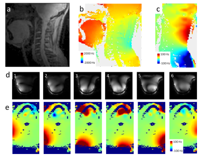
Figure 3 – The 6 channel transceive array facilitates good coverage over the cervical spine (a), although there is a large B0 background field present (b). The transceive array with B0 shim capabilities can provide additional B0 fields (c, sagittal). The six channels show non-overlapping RF fields (d) as well as complementary B0 fields (e) even for 1A current.
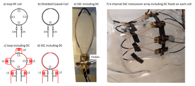
Figure 1 – Extension of RF coils with DC circuits. In a traditional loop coil (a) the conductor is broken up with capacitors whereas (b) shielded coaxial coils (SSC) do not require this. Adding a DC path (red) therefore typically requires the addition of several RF chokes in a traditional coil (c) compared to only two on an SSC coil (d). Addition of RF chokes is only required on the feeding points (e) and not limited additional space is needed on the coil array (f). Note the coil array shows virtually no coupling between the elements despite lack of overlap between elements (data not shown).
-
Improving MRI Near Metal with Local B0 Shimming using a Unified Shim-RF Coil (UNIC): First Case Study, Hip Prosthesis in Phantom.
Fardad Michael Serry1, Junzhou Chen1,2, Anthony G Christodoulou1,2, Yuheng Huang1,2, Fei Han3, Won Bae4,5, Christine Chung4,5, Richard Handlin1, John Stager1, Matthew Dausch1, Yubin Cai1, Yujie Shan1, Yucen Liu1, Yibin Xie1, Xiaoming Bi3, Rohan Dharmakumar1,2, Zhaoyang Fan1,6, Debiao Li1,2, Hsin-Jung Yang1, and Hui Han1
1Biomedical Imaging Research Institute, Cedars-Sinai Medical Center, Los Angeles, CA, United States, 2Department of Bioengineering, UCLA, Los Angeles, CA, United States, 3Siemens Medical Solutions USA, Inc., Los Angeles, CA, United States, 4University of California, San Diego, San Diego, CA, United States, 5VA Medical Center, San Diego, CA, United States, 6University of Southern California Department of Radiology, Los Angeles, CA, United States
Novel unified
coil (UNIC) array 3D B0 shim reduced metal-induced signal void artifact,
increasing the visible area around a hip prosthesis in phantom by up to
50% in some slices. The sequence-agnostic technology was tested with a 3D GRE, generally more susceptible to metal artifact than SE.
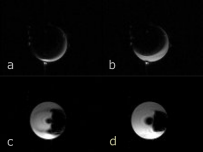
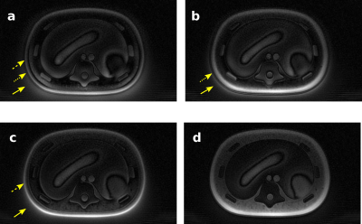
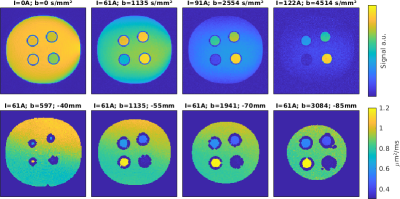
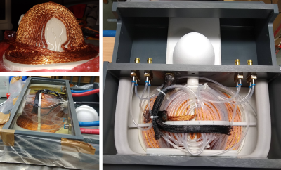
Figure 3. Phantom axial GRE images of cross sections at the femoral head (a,b) and near the femoral insertion end (c,d) of the metal hip prosthesis at TE=4.80ms before (left) and after (right) adding UNIC shim to scanner shim. Signal void is stronger at the longer echo time due to additional dephasing between the two echos. UNIC shimming reduced signal void artifact area by 9% (b versus a) and 9% (d versus c), and extended the visible area closer to the metal, increasing it by 50% (b versus a); and 8 % (d versus c); see text for ROI definition. Fiducial markers are visible in a and b.
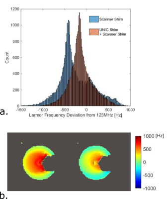
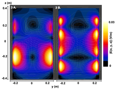
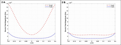
Figure 5. B0 field homogeneity improvement
with UNIC shimming. Histograms of Larmor frequency deviation from the scanner center
frequency (~123MHz), of the masked volume of pixels in the 3D slab scanned before
and after adding UNIC shim to scanner shim (a), and B0 field magnitude maps (b)
for the slice in Figures 3c,d before (b. left) and after (b. right) adding UNIC
shim to scanner shim.
-
Shimming-Toolbox: An open-source software package for performing realtime B0 shimming experiments
Alexandre D'Astous1, Ryan Topfer1, Gaspard Cereza1, Eva Alonso-Ortiz1, Lincoln Craven-Brightman2, Jason Stockmann2,3, and Julien Cohen-Adad1,4
1NeuroPoly Lab, Institute of Biomedical Engineering, Ecole Polytechnique, Montreal, QC, Canada, 2Athinoula A. Martinos Center for Biomedical Imaging, Massachusetts General Hospital, Charlestown, MA, United States, 3Harvard Medical School, Boston, MA, United States, 4Functional Neuroimaging Unit, Centre de recherche de l'Institut universitaire de gériatrie de Montréal, Montreal, QC, Canada
Shimming Toolbox is an open-source software package that aims to provide an easy-to-use, streamlined platform to perform static, dynamic and realtime $$$B_0$$$ shimming experiments.
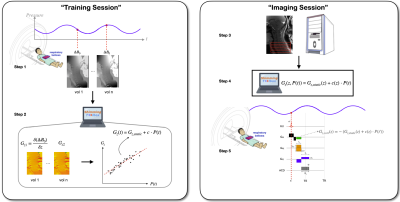
Figure 2: Realtime z-shimming overview. Training session: Step 1: The pressure and fieldmaps are acquired. Step 2: Shimming Toolbox’s optimizer computes a time series of Gz maps. A linear regression is computed between the field gradient and the pressure. Imaging session: Step 3: A dummy GRE scan is run in order to obtain the target image. Step 4: The $$$G_z$$$ maps are resampled onto the target GRE images and $$$G_{z, static}$$$ and c for each slice are sent to the scanner. Step 5: Run the custom realtime z-shimming GRE sequence.
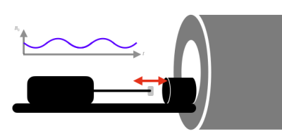
Figure 1: Pneumatic phantom with a long stick, which terminates by a slightly ferromagnetic object that oscillates back and forth creating a time-varying magnetic field.
-
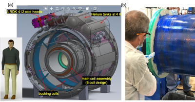
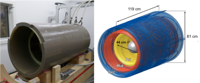
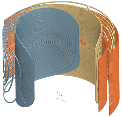
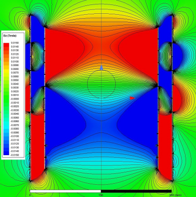
Magnetic fields produced by simple coils inside finite-length cylindrical passive shields with end-caps
Richard W. Bowtell1, Michael Packer 2, Peter Hobson 2, James Leggett1, Niall Holmes1, Paul Glover 1, Matthew Brookes1, and Mark Fromhold2
1Sir Peter Mansfield Imaging Centre, University of Nottingham, Nottingham, United Kingdom, 2School of Physics and Astronomy, University of Nottingham, Nottingham, United Kingdom
We show
how to analytically calculate the fields that are produced by simple coils inside
a finite-length, cylindrical mu-metal shield with end-caps.
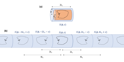
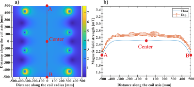
Figure 1
(a) Schematic diagram cylindrical shield with end-caps of radius,
b, and length, 2Ls,
and coil of radius, a. Illustrative coil wirepath and direction of current flow indicated. (b) Multiple reflections
of the coil due to the end-caps (dotted lines indicate reflected versions of the wirepath).
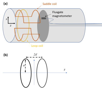
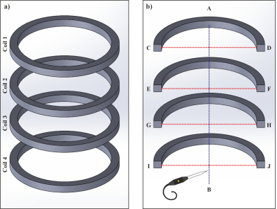
Figure 2 (a) Experimental set-up: fields from loop and saddle coils measured using a fluxgate magnetometer inside a 30 cm diameter 1 m long cylinder formed from 1.5 mm thick mu-metal. (b) Helmholtz-type coil formed from two loops of radius a, separated by a distance 2d, carrying current in the same sense.
-
Hardware developed for phase and frequency locking of interleaved MRI and DMI studies
Terence W. Nixon1, Yanning Liu1, Henk M. DeFeyter1, Scott McIntyre1, and Robin A. de Graaf1
1Yale University, New Haven, CT, United States
Hardware
was developed to allow 2H DMI data to be interleaved into a 1H MRI experiment
thereby reducing scan time. 2H signal was upconverted to and acquired as 1H
data using an RF mixer with a frequency and phased locked local oscillator.
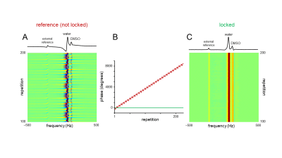
Figure 3 – Phase variation during 2H MRS interleaved with a
7-slice spin-echo MRI. The phantom consisted of three bottles containing ~0.1%
D2O and various amounts of DMSO-D6 (~0.02 – 0.05%). A small (0.5 mL) phantom
containing pure D2O served as an external off-resonance reference signal. (A)
Phase variation in the absence of a phase lock. (B) In addition to the strong
linear phase roll there is also a smaller sequence-dependent phase modulation.
(C) In the presence of a phase lock, each spectrum has an identical phase. The
1D spectra shown in (A) and (C) are extracted from repetition 200.
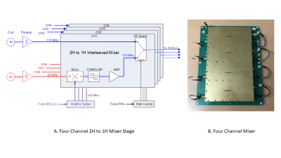
Figure 1 – (A) Four channel interleaved mixer. Inputs for the mixer are from their
respective preamplifiers. The 1H signal is applied to one arm of the RF switch.
The 2H signal is sent to an RF mixer and upconverted to 170MHz by mixing with
the 144MHz LO. The upconverted signal is filtered to remove the unwanted
sideband, amplified and sent to the RF switch. The PPG controls when each nucleus
is sent to the scanner’s 1H receiver. (B) Each channel is isolated from outside
interference and each other by using a dedicated RF shielded enclosure built
onto the board.
-
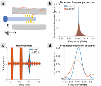
Simultaneous transmit/receive for Bloch-Siegert encoding: a feasibility study
Baosong Wu1, Sajad Hosseinnezhadian2, Yonghyun Ha2, Kartiga Selvaganesan2, Charles Rogers III2, Kasey Hancock2, Gigi Galiana2, and R. Todd Constable2
1Department of Radiology and Biomedical Imaging, Yale School of Medicine, NEW HAVEN, CT, United States, 2Department of Radiology and Biomedical Imaging, Yale School of Medicine, New Haven, CT, United States
The feasibility of simultaneous
transmit/receive was studied at 1MHz. This study demonstrates survival of the NMR
signal in nanovolt level in strong radio frequency
interference.
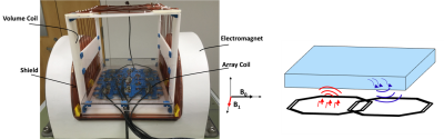
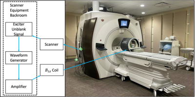
Figure 1. (a) The
open MRI system. (b) The diagram of simultaneous transmit and receive. The phantom is above the
coils. The coil on the right side is for the use of picking up NMR signal at
1MHz, and the coil on the right side is irradiating offset field.
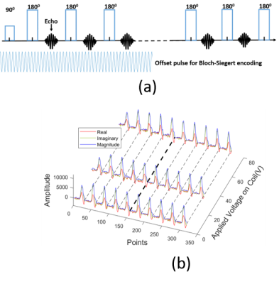
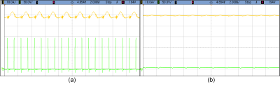
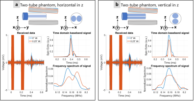
Figure 5. Experiments for simultaneous transmit and
receive. (a) The diagram of a multiple spin echo sequence with continuous
offset irradiation in the front five acquisition window. (b) Experimental data acquired
with the sequence above with echo spacing (TE) 1ms. It shows three echo trains
under different offset-field irradiations.
-
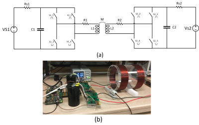
RF sinc pulse distortion compensation using multiple square pulses at 1 MHz.
Yonghyun Ha1, Kartiga Selvaganesan1, Baosong Wu1, Kasey Hancock1, Charles Rogers III1, Sajad Hosseinnezhadian1, Gigi Galiana1, and R. Todd Constable1
1Department of Radiology and Biomedical Imaging, Yale School of Medicine, New Haven, CT, United States
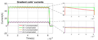
Compensation pulses are shown that were optimized using a series of square
pulses. The SNRs of
the echo signal acquired using compensated pulse was compared with those of
signal obtained with uncompensated pulses and showed significant improvements
of 51.5%.
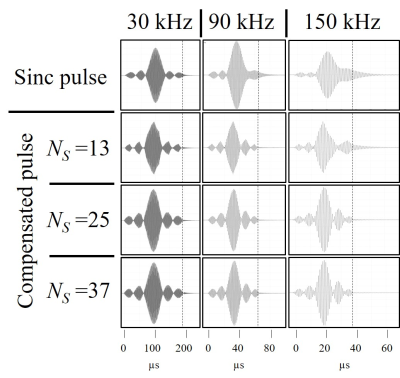
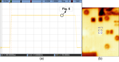
Figure 4. Measured actual pulses (vertical dashed lines indicate the input pulse ends.) of the sinc pulses (top row) and compensated sinc pulses calculated with NS values of 13 (second row), 25 (third row), 37 (bottom row) and bandwidths of 30 kHz (left column), 90 kHz (middle column), and 150 kHz (right column).
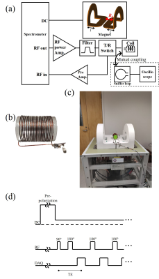
Figure 2. (a) Schematic diagram of an open, table-top, MRI system with photos of (b) the RF solenoid coil and (c) the magnet. (d) A spin-echo sequence with pre-polarization.
-
Automatic 3D B1 field mapping using 3D printer and digital oscilloscope for gradient-free MRI system
Yonghyun Ha1, Kartiga Selvaganesan1, Sajad Hosseinnezhadian1, Baosong Wu1, Kasey Hancock1, Gigi Galiana1, and R. Todd Constable1
1Department of Radiology and Biomedical Imaging, Yale School of Medicine, New Haven, CT, United States
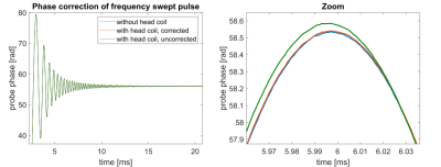
A method to automatically measure the B1 field is introduced.3-axis probe were used to measure the B1 field in three orthogonal axes simultaneously. The position of the probe was controlled by 3D printer, and the peak-to-peak voltage of the signal was automatically saved using oscilloscope.
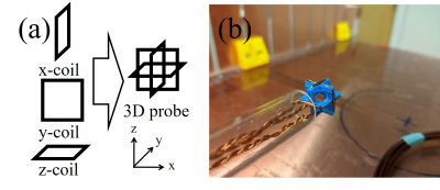
Figure 1. (a) Scheme and (b) photo of the 3-axis probe. The probe consists with three perpendicular square loops.
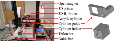
Figure 2. Experimental set up.
-
Inhomogeneity and ramping effects in field-cycled quantitative molecular MRI
Matthew A. McCready1, William B. Handler1, Francisco Martinez2,3, Timothy J. Scholl2,3, and Blaine A. Chronik1,2
1Physics and Astronomy, Western University, London, ON, Canada, 2Medical Biophysics, Western University, London, ON, Canada, 3Robarts Research Institute, Western University, London, ON, Canada
The dreMR method assumes field strength is homogenous and coils reach field instantly. We have shown that these assumptions result in errors within dreMR images, which can be solved by use of improved homogeneity coils and higher slew rates.
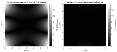
Figure
2. (LEFT) Percent difference in dreMR image of VivoTrax, in uniform
concentration of 160 μM, using field of previously constructed coil. Percent
difference is taken from center point where field is at desired value. (RIGHT) Same
simulation using field from new design method coil. Colour axis chosen to match
the left.
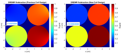
Figure 1. (LEFT) Simulated dreMR image of 4 cylinders of VivoTrax, in concentrations of 20, 80, 120, and 160 μM, using field of previously constructed coil. Note change in signal across cylinders. Sequence uses 300mT field shift in a 0.5T system. (RIGHT) Same simulation using field from new design method coil. Signal does not noticeably change across cylinders. Data points are given in both figures at locations with no contrast agent.
-
Very low field MRI for brain imaging
Samson Lecurieux Lafayette1 and Claude Fermon1
1SPEC - CEA Saclay - Université Paris Saclay, Saclay, France
We have
developed a MRI device working at 10mT for brain imaging. Parallel acquisition
and rapid sequences have been implemented in order to speed up the acquisition
time. Strengths and limitations compared to high field are given.
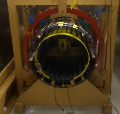
Figure 3: The very low field MRI in the magnetically shielded room.
Figure 1: The eight channels sensor. Each channel is
matched and tuned, and decoupled from emission radiofrequency.
-
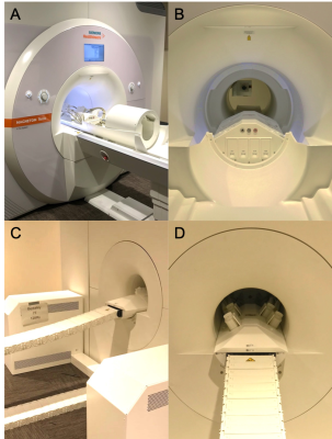
Comparison of SNR between a low-field (0.26T) Tabletop-MRI and a clinical high-field (3T) scanner
Robert Kowal1, Enrico Pannicke2, Marcus Prier1, Ralf Vick2, Georg Rose3, and Oliver Speck1
1Department of Biomedical Magnetic Resonance, Otto von Guericke University, Magdeburg, Germany, 2Chair of Electromagnetic Compatibility, Otto von Guericke University, Magdeburg, Germany, 3Chair in Healthcare Telematics and Medical Engineering, Otto von Guericke University, Magdeburg, Germany
A low-field (0.26T) Tabletop-MR-system was compared to a high-field (3T) clinical scanner by evaluating the SNR of simple FID time domain signals. Direct comparison of the SNR led to a measured relative performance of 11.3% for the Tabletop before compensation for experimental conditions.
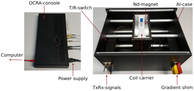
Measurement setup on the Tabletop-system. Left side: OCRA-console for controlling the system, supplying the components and connecting to the computer. Right side: Opened system with the sample in the carrier between the neodymium magnets with connected signal and shimming lines.
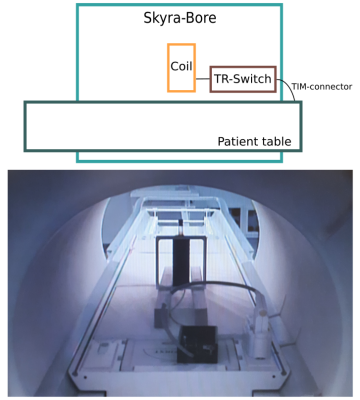
Measurement setup on the Skyra-system. The test tube sample was positioned with the coil perpendicular to the static magnetic �field �fixed by wooden planks on the patient table. The connection to the MR system was established via the T/R-switch and TIM-connector. Shown on the bottom is an image taken with the patient camera.
-
Initial Experience of Body Imaging at 5T
Zhenhua Shen1, Xuchen Zhu1, Shihong Han1, Fuyi Fang1, Wei Luo1, Shao Che1, Zidong Wei1, Jinguang Zong1, Yongquan Ye2, Bo Li1, Shuheng Zhang1, Anthony Vu2, Weiguo Zhang2, and Guobin Li1
1United Imaging Healthcare, Shanghai, China, 2UIH America, Inc., Houston, TX, United States
With
multi-channel RF parallel transmission hardware architecture and static RF shimming
techniques, the uniformity of the RF transmission field is shown to be well
controlled for imaging quality guarantee. Preliminary results show great promise
for body imaging at 5T.
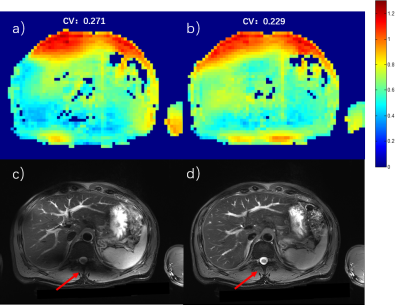
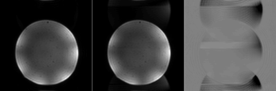
Figure 2 Abdominal imaging at 5T. a) and c) B1+ sensitivity map and T2W FSE image with CP mode excitation. b) and d) B1+sensitivity map and T2W FSE image after static RF shimming optimization. The CV values were measured for bothcases.The red arrows show the most significant improvement area.
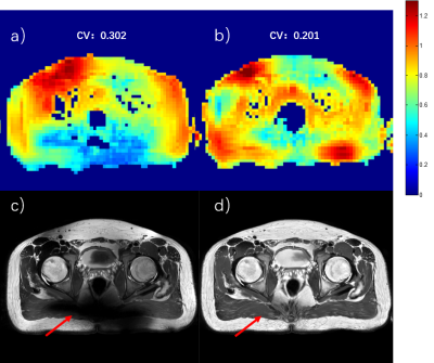
Figure 3 Pelvic imaging at 5T. a) and c) B1+ sensitivity map and T2W FSE image with CP mode excitation. b) and d) B1+sensitivity map and T2W FSE image after static RF shimming optimization. The CV values were measured for bothcases.The red arrows show the most significant improvement area.
-
A sample temperature control system for post mortem MRI
Sebastian Walter Rieger1, Karla Miller1, Peter Jezzard1, and Wenchuan Wu1
1Wellcome Centre for Integrative Neuroimaging, University of Oxford, Oxford, United Kingdom
In
post mortem MRI, RF absorption can cause significant heating in the sample. This
can interfere with scanning and accelerate decomposition of unfixed samples. Here,
a temperature control system is presented which enables prolonged scanning at a
stable temperature while preserving tissue.
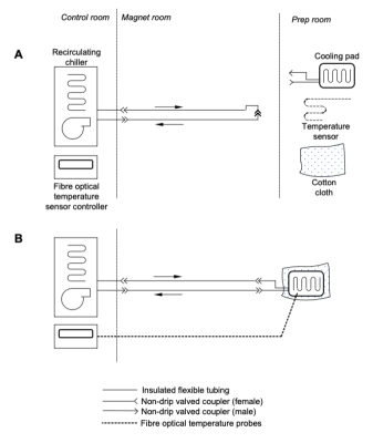
Cooling
system schematic. A: Pre-cooling / setup configuration - The chiller is
operating and pre-cooling the bulk of the fluid to the desired temperature,
while the cooling pad and temperature sensor(s) are being used for sample
preparation. B: Normal operation configuration - The temperature probe(s)
are affixed to the sample, and the cooling pad is wrapped around it. A layer of
cloth around the outside provides thermal insulation to prevent excessive
condensation, and the pad is connected to the chiller.
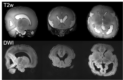
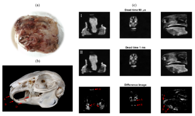
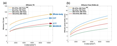
Example T2- and diffusion
weighted images. Top: T2 weighted images were acquired
at 0.4mm isotropic resolution using a 3D-SPACE sequence with FOV=150x150x96mm3,
TR/TE=2300/586ms, 6 repetitions. Bottom: averaged diffusion weighting images
acquired at 0.8mm isotropic resolution using a spin-echo diffusion weighted
readout-segmented EPI sequence with FOV=150x150x104mm3,
TR/TE=10.8s/113ms, multiband factor 2, GRAPPA factor 2, b=9000 s/mm2.
-
Compact MRI bioreactor for real-time monitoring 3D printed tissue-engineered constructs.
Jean-Lynce GNANAGO1,2,3,4,5,6, Tony GERGES1,2,3,4,5,6, Laura Chastagnier1,2,4,6,7,8,9,10, Emma Petiot2,4,6,7,8,9,10, Vincent SEMET1,2,4,5,6, Philippe Lombard1,2,3,4,5,6, Christophe Marquette1,2,4,6,7,8,9,10, Michel Cabrera1,2,3,4,5,6, and Simon Auguste Lambert1,2,3,4,5,6
1Université Claude Bernard Lyon 1, VILLEURBANNE, France, 2INSA LYON, VILLEURBANNE, France, 3Ecole Centrale Lyon, Ecully, France, 4CNRS, VILLEURBANNE, France, 5AMPERE UMR 5005, VILLEURBANNE, France, 6Université de Lyon, VILLEURBANNE, France, 73d.FAB, VILLEURBANNE, France, 8CPE Lyon, VILLEURBANNE, France, 9ICBMS, VILLEURBANNE, France, 10UMR 5246, VILLEURBANNE, France
An MRI bioreactor is built using novel 3D printing techniques and plastronics. The integration of an MRI probe function within the bioreactor opens up possibilities of real time monitoring in the tissue engineering field.
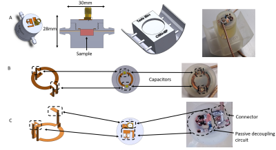
Figure
1: Design and conception of the bioreactor. (A) 3D model of the bioreactor and its support.
(B)
Detailed view of the bottom of the 3D coil
circuit and its integration. (C) Detailed view of the top of the 3D coil
circuit and its integration
Figure
3: (A) Picture of the bioprinted tissue after construction. (B) 2D
TURBO RARE image of the tissue using
the bioreactor acquired on a 7T MRI scanner with
a 75 µm in plane resolution.
-
Characterization of 3AM diffusion MRI phantoms via microscopy, and phase-contrast micro-CT
Farah Mushtaha1,2, Tristan K. Kuehn1,3, Omar El-Deeb4, Seyed A. Rohani3, Luke W. Helpard3, Hanif Ladak2,3,5, Amanda Moehring6, Corey A. Baron1,2,3,7, and Ali R. Khan1,2,3,7
1Robarts Research Institute, London, ON, Canada, 2Medical Biophysics, Schulich School of Medicine and Dentistry, Western University, London, ON, Canada, 3School of Biomedical Engineering, Western University, London, ON, Canada, 4Neuroscience, Western University, London, ON, Canada, 5Department of Electrical and Computer Engineering, Western University, London, ON, Canada, 6Biology, Western University, London, ON, Canada, 7The Brain and Mind Institute, Western University, London, ON, Canada
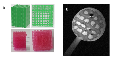
Pore diameters of the 3AM phantoms measured using microscopy and micro-CT were in agreement with a mean pore diameter of ~ 8 μm, and fits of both kurtosis and ball and stick models were in agreement between simulation and acquired dMRI data.
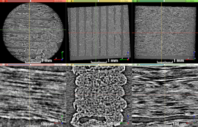
Figure 3. Synchrotron micro-CT scan data at two zoom levels, transformed to align lines of material with the viewing planes. Upper row: View of the entire scan ROI. Lower row: Detailed view of a short length of five stacked lines of material. The direction of print-head motion was left-right in the left- and right-most columns, and perpendicular to the image in the center column.
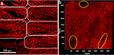
Figure 1. a) Confocal microscopy z-stack image of a stained phantom slide. Elastomeric matrix (red) and pores (black) are visible. Each white outline indicates an individual line of material. b) 2D projection of a 3D microscopy volume acquired with confocal microscopy. Outlined in yellow are larger pores caused by the printing pattern of the phantom. In both a and b, the image plane is perpendicular to the long axis of the pores.
-
A phantom system for evaluating the effect of lipid and iron composition on qMRI parameters
Rona Shaharabani1, Shir Filo1, Oshrat Shtangel1, and Aviv Mezer1
1The Edmond and Lily Safra Center for Brain Science, The Hebrew University of Jerusalem, Jerusalem, Israel, Jerusalem, Israel
We describe a phantom system composed of lipids and iron for the assessment of their unique contribution to quantitative MRI parameters. We found that both changes in lipid concentrations (lipid-water fraction) and iron concentrations affected R2*, for all lipid types.
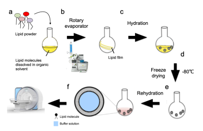
Fig. 1: Schematic representation of the MLV preparation method. (a) Soy PC, alone or as a mixture, was dissolved in chloroform (b) put in a vacuum rotary evaporator to create a uniform lipid film. (c) Ammonium bicarbonate was added to dissolve the lipid film. (d) The solution was then lyophilized and (e) rehydrated with a desired iron ion buffer to create the iron ion encapsulated MLV. (f) The samples were imaged in a clinical scanner.
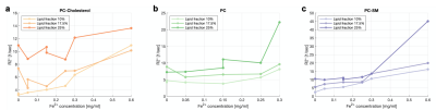
Fig. 3: qMRI relaxation rate R2* with increasing concentration of iron ion Fe2+. R2* is affected by the lipid-water fraction and iron concentration. R2* values increase with increasing concentration of Fe2+ for all lipid types. Each color represents a different lipid-water fraction MLV phantom. (a) Lipid MLV phantom PC-Cholesterol with Fe2+. (b) Lipid MLV phantom PC with Fe2+. (c) Lipid MLV phantom PC-SM with Fe2+.