Systems Engineering II
Engineering/Interventional/Safety Wednesday, 19 May 2021
Oral

Oral Session - Systems Engineering II
Engineering/Interventional/Safety
Wednesday, 19 May 2021 18:00 - 20:00
  • Approaching Real-Time Patient-Specific SAR Calculation for Parallel Transmission at 7 Tesla
    Eugene Milshteyn1,2, Georgy Guryev3, Angel Torrado-Carvajal1,2,4, Jacob K. White3, Lawrence L. Wald1,2,5, and Bastien Guerin1,2
    1Athinoula A. Martinos Center for Biomedical Imaging, Charlestown, MA, United States, 2Harvard Medical School, Boston, MA, United States, 3Dept. of Electrical Engineering and Computer Science, Massachusetts Institute of Technology, Cambridge, MA, United States, 4Medical Image Analysis and Biometry Laboratory, Universidad Rey Juan Carlos, Madrid, Spain, 5Harvard-MIT Division of Health Sciences and Technology, Cambridge, MA, United States
    This study focuses on developing a fast methodology for patient-specific SAR calculations with an 8 channel pTx head coil at 7T. This methodology consists of fast acquisition, segmentation, and electromagnetic analysis.
    Figure 1: A. Flow chart depicting our methodology for fast computation of the patient-specific B1+ and SAR maps. B. 7T 8 channel pTx coil model simulated in this work and loaded with a body model for one of the volunteers. The body is extended 100 mm beyond the edge of the coil to eliminate any potential current “pseudo-loops” (11) that would affect the electromagnetic calculations.
    Figure 4: Simulated and acquired B1+ maps for all 8 channels for three of the volunteers. While the simulated coil was not the same as the coil used for acquisition, both are 8 channel coils that comfortably conform to the volunteer head. The magnitude intensities shown were normalized. Qualitatively, the maps match up in terms of magnetic field distribution within the head. Future work will focus on being able to simulate and acquire with the same coil, which will allow more direct comparison of B1+ maps between simulation and acquisition, and be used as verification of the methodology.
  • Rapid calibration scan for estimating temporally-varying eddy currents in diffusion imaging using a time-resolved PEPTIDE imaging approach
    Merlin J Fair1 and Kawin Setsompop1,2
    1Radiological Sciences Laboratory, Stanford University, Stanford, CA, United States, 2Electrical Engineering, Stanford University, Stanford, CA, United States
    The time-resolved PEPTIDE approach is investigated for use as a fast (<30s) calibration scan for the estimation of eddy current induced phase evolutions. Simulation, phantom and in vivo work demonstrates the potential accuracy of such a technique, including up to a b-value of 5000s/mm2.
    Figure 5 – (a) Single-shot data: phantom & in-vivo. The low SNR of b=5000 in-vivo data is apparent in both EPI and PEPTIDE (PEP), but image phase across time is still measurable. (b) Estimated phantom eddy fields, measured by FSL and PEPTIDE. First 3 directions for PEPTIDE are direct estimates (red square), while others are calculated using a linear model. (c) Estimated in-vivo eddy fields (with same diffusion-directions and acq. params as in phantom). “Phantom PEP-ref”: PEPTIDE-estimated field in the phantom, masked by the in-vivo brain FOV, for reference with the in-vivo results.
    Figure 1 - a) EPTI/PEPTIDE uses a zig-zag sampling trajectory to cover a large ky-t section per acquisition shot, with B0-informed-GRAPPA used to fill-in the missing data. PEPTIDE acquires rotated EPTI shots (blades) to cover the full k-t space. With full k-t data, each time-point has consistent phase and signal decay, so the images in the resolved time-series are free from typical-EPI distortion and blurring. b) The phase of the time-series images for a DWI acquisition can be compared with that of a diffusion-free (b=0) acquisition, to estimate eddy current induced phase changes.
  • Fully Integrated Scanner Implementation of Direct Signal Control for 2D T2-Weighted TSE at Ultra-High Field
    Raphael Tomi-Tricot1,2,3, Jan Sedlacik2,3, Jonathan Endres4, Juergen Herrler5, Patrick Liebig6, Rene Gumbrecht6, Dieter Ritter6, Tom Wilkinson2,3, Pip Bridgen7, Sharon Giles7, Armin M. Nagel4, Joseph V. Hajnal2,3, Radhouene Neji1,2, and Shaihan J. Malik2,3
    1MR Research Collaborations, Siemens Healthcare Limited, Frimley, United Kingdom, 2Biomedical Engineering Department, School of Biomedical Engineering and Imaging Sciences, King's College London, London, United Kingdom, 3Centre for the Developing Brain, School of Biomedical Engineering and Imaging Sciences, King's College London, London, United Kingdom, 4Institute of Radiology, University Hospital Erlangen, Erlangen, Germany, 5Institute of Neuroradiology, University Hospital Erlangen, Erlangen, Germany, 6Siemens Healthcare GmbH, Erlangen, Germany, 7School of Biomedical Engineering and Imaging Sciences, King's College London, London, United Kingdom
    Direct Signal Control was successfully applied in the brain at 7T in routine conditions and without manual intervention. It consistently achieved higher and more homogeneous signal in T2-weighted FSE sequences, under strict SAR limits.
    Figure 4: For each subject (rows), comparison of images acquired with static RF shimming (RFShim) and direct signal control (DSC) in two representative slices (groups A and B). DSC shows improved signal homogeneity compared to RFShim in cerebellum and lower brain cortex. Arrowheads point at some areas of interest (DSC gain in green, loss in red).
    Figure 5: For each subject, maps of relative signal difference ($$$\delta{S}$$$) between RFShim and DSC on four representative slices, and histogram of $$$\delta{S}$$$ on the whole brain. Regions exhibiting signal differences beyond +20% (resp. -20%) are highlighted in green (resp. red). Only in Subject 4 signal loss is observed in central brain despite B1+ correction; other regions see a net signal gain with DSC . Average $$$\delta{S}$$$ is reported on histograms. Also note the agreement with the last row of Figure 3 (Subject 3).
  • Frequency Drift in MR Spectroscopy: An 87-scanner 3T Phantom Study
    Steve C.N. Hui1,2, Mark Mikkelsen1,2, Helge J. Zöllner1,2, Vishwadeep Ahluwalia3, Sarael Alcauter4, Laima Baltusis5, Deborah A. Barany6, Laura R. Barlow7, Robert Becker8, Jeffrey I. Berman9, Adam Berrington10, Pallab K. Bhattacharyya11, Jakob Udby Blicher12, Wolfgang Bogner13, Mark S. Brown14, Vince D. Calhoun15, Ryan Castillo16, Kim M. Cecil17, Yeo Bi Choi18, Winnie C.W. Chu19, William T. Clarke20, Alexander R. Craven21, Koen Cuypers22, Michael Dacko23, Camilo de la Fuente-Sandoval24, Patricia Desmond25, Aleksandra Domagalik26, Julien Dumont27, Niall W. Duncan28, Ulrike Dydak29, Katherine Dyke30, David A. Edmondson17, Gabriele Ende8, Lars Ersland31, C. John Evans32, Alan S. R. Fermin33, Antonio Ferretti34, Ariane Fillmer35, Tao Gong36, Ian Greenhouse37, James T. Grist38, Meng Gu39, Ashley D. Harris40, Katarzyna Hat41, Stefanie Heba42, Eva Heckova13, John P. Hegarty II43, Kirstin-Friederike Heise44, Aaron Jacobson45, Jacobus F.A. Jansen46, Christopher W. Jenkins47, Stephen J. Johnston48, Christoph Juchem49, Alayar Kangarlu50, Adam B. Kerr5, Karl Landheer51, Thomas Lange52, Phil Lee53, Swati Rane Levendovszky54, Catherine Limperopoulos55, Feng Liu56, William Lloyd57, David J. Lythgoe58, Maro G. Machizawa59, Erin L. MacMillan7, Richard J. Maddock60, Andrei V. Manzhurtsev61, María L. Martinez-Gudino62, Jack J. Miller63, Heline Mirzakhanian64, Paul G. Mullins65, Jamie Near66, Wibeke Nordhøy67, Georg Oeltzschner1,2, Raul Osorio62, Maria C.G. Otaduy68, Erick H. Pasaye4, Ronald Peeters69, Scott J. Peltier70, Ulrich Pilatus71, Nenad Polomac71, Eric C. Porges72, Subechhya Pradhan55, James Joseph Prisciandaro73, Nick Puts74, Caroline D. Rae75, Francisco Reyes-Madrigal76, Timothy P.L. Roberts9, Caroline E. Robertson77, Muhammad G. Saleh78, Jens T. Rosenberg79, Diana-Georgiana Rotaru58, O'Gorman Tuura L. Ruth80, Kristian Sandberg12, Ryan Sangill81, Keith Schembri82, Anouk Schrantee83, Natalia A. Semenova84, Debra Singel85, Rouslan Sitnikov86, Jolinda Smith87, Yulu Song36, Craig Stark88, Diederick Stoffers89, Stephan P. Swinnen44, Costin Tanase60, Sofie Tapper1,2, Martin Tegenthoff42, Thomas Thiel90, Marc Thioux91, Peter Truong92, Pim van Dijk91, Nolan Vella82, Rishma Vidyasagar93, Andrej Vovk94, Guangbin Wang36, Lars T. Westle67, Timothy K. Wilbur54, William R. Willoughby95, Martin Wilson96, Hans-Jörg Wittsack97, Adam J. Woods98, Yen-Chien Wu99, Junqian Xu100, Maria Yanez Lopez101, David K.W. Yeung19, Qun Zhao102, Xiaopeng Zhou29, Gasper Zupan94, and Richard A.E. Edden1,2
    1Russell H. Morgan Department of Radiology and Radiological Science, The Johns Hopkins University School of Medicine, Baltimore, MD, United States, 2F.M. Kirby Research Center for Functional Brain Imaging, Kennedy Krieger Institute, Baltimore, MD, United States, 3GSU/GT Center for Advanced Brain Imaging, Georgia Institute of Technology, Atlanta, GA, United States, 4Instituto de Neurobiología, Universidad Nacional Autónoma de México, Queretaro, Mexico, 5Center for Cognitive and Neurobiological Imaging, Stanford University, Stanford, CA, United States, 6Kinesiology, University of Georgia, Athens, GA, United States, 7Department of Radiology, The University of British Columbia, Vancouver, BC, Canada, 8Center for Innovative Psychiatry and Psychotherpay Research, Department Neuroimaging, Central Institute of Mental Health, Medical Faculty Mannheim, Heidelberg University, Mannheim, Germany, 9Department of Radiology, Children's Hospital of Philadelphia, Philadelphia, PA, United States, 10Sir Peter Mansfield Imaging Centre, School of Physics and Astronomy, University of Nottingham, Nottingham, United Kingdom, 11Imaging Institute, The Cleveland Clinic, Cleveland, OH, United States, 12Center of Functionally Integrative Neuroscience, Aarhus University, Aarhus, Denmark, 13Department of Biomedical Imaging and Image-guided Therapy, High-Field MR Center, Medical University of Vienna, Vienna, Austria, 14Department of Radiology, University of Colorado Anschutz Medical Campus, Aurora, CO, United States, 15Tri-Institutional Center for Translational Research in Neuroimaging and Data Science(TReNDS), Georgia State University, Georgia Institute of Technology, and Emory University, Atlanta, GA, United States, 16Neuroscience Research AustraliaNeuRA Imaging, Randwick, Australia, 17Department of Radiology, Cincinnati Children's Hospital Medical Center, Cincinnati, OH, United States, 18Psychological and Brain Sciences, Dartmouth College, Hanover, NH, United States, 19Department of Imaging & Interventional Radiology, The Chinese University of Hong Kong, Hong Kong, Hong Kong, 20Wellcome Centre for Integrative Neuroimaging, NDCN, University of Oxford, Oxford, United Kingdom, 21Department of Biological and Medical Psychology, University of Bergen, Haukeland University Hospital, Bergen, Norway, 22REVAL Rehabilitation Research Institute (REVAL), Hasselt University, Diepenbeek, Belgium, 23Department of Radiology, Medical Physics, Medical Center - University of Freiburg, Faculty of Medicine, University of Freiburg, Freiburg, Germany, 24Laboratory of Experimental Psychiatry & Neuropsychiatry Department, Instituto Nacional de Neurología y Neurocirugía, Mexico City, Mexico, 25Department of Radiology, University of Melbourne/ Royal Melbourne Hospital, Melbourne, Australia, 26Malopolska Centre of Biotechnology, Jagiellonian University, Krakow, Poland, 27Clinical Imaging Core Facility, CI2C Lille, Lille, France, 28Graduate Institute of Mind, Brain and Consciousness, Taipei Medical University, Taipei, Taiwan, 29School of Health Sciences, Purdue University, West Lafayette, IN, United States, 30School of Psychology, University of Nottingham, Nottingham, United Kingdom, 31Department of Clinical Engineering, University of Bergen, Haukeland University Hospital, Bergen, Norway, 32CUBRIC, Cardiff University, Cardiff, United Kingdom, 33Center for Brain, Mind and Kansei Sciences Research, Hiroshima University, Hiroshima, Japan, 34Neuroscience, Imaging and Clinical Sciences, University "G. d'Annunzio" of Chieti-Pescara, Chieti, Italy, 35Physikalisch-Technische Bundesanstalt (PTB), Braunschweig und Berlin, Germany, 36Department of Imaging and Nuclear Medicine, Shandong Medical Imaging Research Institute, Shandong University, Jinan, China, 37Human Physiology, University of Oregon, Eugene, OR, United States, 38Physiology, Anatomy, and Genetics/ Oxford Centre for Magnetic Resonance, The University of Oxford / Department of Radiology, The Churchill Hospital, The University of Oxford, Oxford, United Kingdom, 39Department of Radiology, Stanford University, Stanford, CA, United States, 40Department of Radiology, University of Calgary, Calgary, AB, Canada, 41Institute of Psychology, Jagiellonian University, Krakow, Poland, 42Department of Neurology, BG University Hospital Bergmannsheil, Bochum, Germany, 43Psychiary & Behavioral Sciences, Stanford University, Stanford, CA, United States, 44Department of Movement Sciences, KU Leuven, Leuven, Belgium, 45Department of Radiology, University of California San Diego, San Diego, CA, United States, 46Department of Radiology and Nuclear Medicine, Maastricht University Medical Center, Maastricht, Netherlands, 47CUBRIC, Cardiff university, Cardiff, United Kingdom, 48Psychology Dept. / Clinical Imaging Facility, Swansea University, Swansea, United Kingdom, 49Biomedical Engineering and Radiology, Columbia University, New York City, NY, United States, 50Psychiatry, Columbia University Irving Medical Center/New York State Psychiatric Institute, New York City, NY, United States, 51Biomedical Engineering, Columbia University, New York City, NY, United States, 52Department of Radiology, Medical Physics, University of Freiburg, Freiburg, Germany, 53Department of Radiology, University of Kansas Medical Center, Kansas, KS, United States, 54Department of Radiology, University of Washington, Seattle, WA, United States, 55Developing Brain Institute, Diagnostic Imaging and Radiology, Children's National Hospital, Washington, DC, United States, 56Department of Psychiatry, Columbia University Irving Medical Center/New York State Psychiatric Institute, New York, NY, United States, 57Division of Informatics, Imaging & Data Sciences, University of Manchester, Manchester, United Kingdom, 58Department of Neuroimaging, King's College London, London, United Kingdom, 59Center for Brain, Mind and KANSEI Sciences Research, Hiroshima University, Hiroshima, Japan, 60Psychiatry and Behavioral Sciences, University of California Davis, Imaging Research Center, Davis, CA, United States, 61Department of Radiology, Clinical and Research Institute of Emergency Pediatric Surgery and Trauma, Moscow, Russian Federation, 62Imágenes Cerebrales, Instituto Nacional de Psiquiatría Ramón de la Fuente, Mexico City, Mexico, 63Department of Physics, University of Oxford, Oxford, United Kingdom, 64Department of Psychiatry, University of California San Diego, San Diego, CA, United States, 65Department of Psychology, Bangor University, Bangor, United Kingdom, 66Douglas Mental Health University Institute and Department of Psychiatry, McGill University, Montreal, QC, Canada, 67Department of Diagnostic Physics, Division of Radiology and Nuclear Medicine, Oslo University Hospital, Oslo, Norway, 68LIM44, Instituto e Departamento de Radiologia, Faculdade de Medicina, Universidade de Sao Paulo, Sao Paulo, Brazil, 69Department of Imaging & Pathology, Department of Radiology, University Hospitals Leuven, KU Leuven, Leuven, Belgium, 70Functional MRI Laboratory, University of Michigan, Ann Arbor, MI, United States, 71Institute of Neuroradiology, Goethe-University Frankfurt, Frankfurt, Germany, 72Center for Cognitive Aging and Memory, McKnight Brain Institute, Department of Clinical and Health Psychology, College of Public Health and Health Professions, University of Florida, Gainesville, FL, United States, 73Psychiatry and Behavioral Sciences, Medical University of South Carolina, Charleston, SC, United States, 74Forensic & Neurodevelopmental Sciences, King's College London, London, United Kingdom, 75NeuRA Imaging, Neuroscience Research Australia, Randwick, Australia, 76Laboratory of Experimental Psychiatry, Instituto Nacional de Neurología y Neurocirugía, Mexico City, Mexico, 77Department of Psychological and Brain Sciences, Dartmouth College, Hanover, NH, United States, 78Department of Diagnostic Radiology and Nuclear Medicine, University of Maryland School of Medicine, Baltimore, MD, United States, 79McKnight Brain Institute, AMRIS, University of Florida, Gainesville, FL, United States, 80Center for MR Research, University Children's Hospital, Zurich, Switzerland, 81Center of Functionally Integrative Neuroscience, Aarhus University Hospital, Aarhus, Denmark, 82Medical Physics, Mater Dei Hospital, Imsida, Malta, 83Department of Radiology and Nuclear Medicine, Amsterdam University Medical Center, University of Amsterdam, Amsterdam, Netherlands, 84504, Emanuel Institute of Biochemical Physics of the Russian Academy of Sciences, Moscow, Russian Federation, 85Psychiatry, University of Colorado Anschutz Medical Campus, Aurora, CO, United States, 86Clinical Neuroscience, MRI Centre, Karolinska Institutet, Clinical Neuroscience, MRI Centre, Sweden, 87Lewis Center for Neuroimaging, University of Oregon, Eugene, OR, United States, 88Department of Neurobiology and Behavior, Facility for Imaging and Brain Research (FIBRE) & Campus Center for Neuroimaging (CCNI), University of California, Irvine, Irvine, CA, United States, 89Spinoza Centre for Neuroimaging, Royal Netherlands Academy of Arts and Sciences, Amsterdam, Netherlands, 90Institute of Clinical Neuroscience and Medical Psychology, University Dusseldorf, Medical Faculty, Düsseldorf, Germany, 91Otorhinolaryngology, Head and Neck Surgery, University of Groningen, University Medical Center Groningen, Groningen, Netherlands, 92Brain Health Imaging Centre, Centre for Addiction and Mental Health, Toronto, ON, Canada, 93Melbourne Dementia Research Centre, Florey Institute of Neurosciences and Mental Health, Melbourne, Australia, 94Faculty of Medicine, University of Ljubljana, Ljubljana, Slovenia, 95Department of Radiology, University of Alabama at Birmingham, Birmingham, AL, United States, 96Centre for Human Brain Health, University of Birmingham, Birmingham, United Kingdom, 97Department of Diagnostic and Interventional Radiology, University Dusseldorf, Medical Faculty, Düsseldorf, Germany, 98Center for Cognitive Aging and Memory, McKnight Brain Institute, Department of Clinical and Health Psychology, College of Public Health and Health Professions. Department of Neuroscience, College of Medicine, University of Florida, Gainesville, FL, United States, 99Department of Radiology, TMU-Shuang Ho Hospital, New Taipei City, Taiwan, 100Department of Radiology and Psychiatry, Baylor College of Medicine, Houston, TX, United States, 101Perinatal Imaging & Health, King's College London, London, United Kingdom, 102Bioimaging Research Center, University of Georgia, Athens, GA, United States
    This study measured field drift in eighty-seven 3T scanners using the water signal acquired by MRS. Frequency traces were plotted for each dynamic and severity of drift quantified. This dataset will be publicly available for benchmark and further analyses.
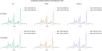
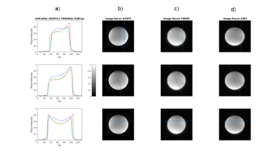
    Figure 4. Comparison of simulated spectra with frequency drift applied between minimum and maximum drift for pre- and post-fMRI PRESS data. The minimum-drift case for each vendor (50% opacity) is overlaid with the maximum-drift case (opaque).
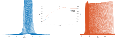
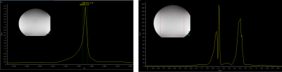
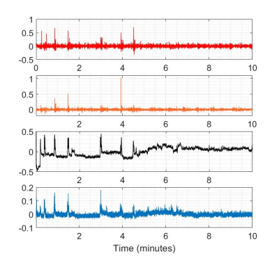
    Figure 1. Individual transients of pre- and post-fMRI PRESS (plotted in blue and red, respectively) from the highest-drifting scanner. The frequency offset derived from modeling the water signals is plotted (middle). 360 averages correspond to 30 minutes total scan duration.
  • A 64-Channel Brain Array Coil with an Integrated 16-Channel Field Monitoring System for 3T MRI
    Mirsad Mahmutovic1, Alina Scholz1, Nicolas Kutscha1, Markus W. May1, Torsten Schlumm2, Roland Müller2, Kerrin Pine2, Luke J. Edwards2, Nikolaus Weiskopf2,3, David O. Brunner4, Harald E. Möller2, and Boris Keil1
    1Institute of Medical Physics and Radiation Protection, TH Mittelhessen University of Applied Sciences, Giessen, Germany, 2Max Planck Institute for Human Cognitive and Brain Sciences, Leipzig, Germany, 3Felix Bloch Institute for Solid State Physics, Faculty of Physics and Earth Sciences, Leipzig University, Leipzig, Germany, 4Skope Magnetic Resonance Technologies AG, Zurich, Switzerland
    The constructed 64-channel brain coil with integrated 16-channel field monitoring system provided enhanced reception sensitivity and encoding power. The combination with strong gradients will improve diffusion-weighted imaging (DWI).
    Constructed 64-channel array coil with an incorporated 16-channel field camera system. (a) 3D model of the coil, (b) enclosed finished coil, (c) view into the open coil.
    (A) Zero-order phase and higher-order dynamic dynamic field effects; (B) first-order read trajectory. Examples of tSNR maps (calculated from series of 20 repetitions) obtained with the 64ch coil and (C) spiral as well as (D) EPI acquisitions. Images reconstructed from the spiral acquisitions using concurrently monitored field information do not show evident distortions at visual inspection. (E) Corresponding results obtained with EPI and the standard 32ch coil are shown for comparison. Note the SNR gain obtained with the 64ch coil, in particular in cortical regions.
  • MaxGIRF: Image Reconstruction Incorporating Maxwell Fields and Gradient Impulse Response Function Distortion
    Nam G. Lee1, Rajiv Ramasawmy2, Adrienne E. Campbell-Washburn2, and Krishna S. Nayak1,3
    1Biomedical Engineering, University of Southern California, Los Angeles, CA, United States, 2Cardiovascular Branch, Division of Intramural Research, National Heart, Lung, and Blood Institute, National Institutes of Health, Bethesda, MD, United States, 3Ming Hsieh Department of Electrical and Computer Engineering, University of Southern California, Los Angeles, CA, United States
    We present MaxGIRF, an image reconstruction method to simultaneously mitigate local blurring caused by concomitant fields and static off-resonance. We demonstrate successful application to 2D spin-echo spiral brain imaging at 0.55T with (long) 12ms readouts.
    Figure 1. Flowchart of the proposed MaxGIRF reconstruction. (A) Logical gradient waveforms are first transformed to the physical coordinate system (PCS). Gradient inaccuracies in PCS are estimated using phantom-based GIRFs. Analytic expressions of concomitant fields are then derived from the coil geometry, presumed gradient non-linearity, and GIRF-predicted gradients, for each spatial position in PCS. (B) The phase evolution per voxel is represented as the sum of phase contributions from static off-resonance (red) and linear gradients and concomitant field terms (blue).

    Figure 4. Multi-slice axial spiral imaging of a healthy volunteer at 0.55T. (left) CG-SENSE reconstructions; (middle) MaxGIRF reconstructions without static off-resonance correction (i.e., without a field map); (right) Absolute difference images. GIRF-predicted gradients were used in bothreconstructions. The improvement in concomitant field blurring is evident in away from isocenter, as expected. Static off-resonance correction was not performed, in order to isolate the difference due to concomitant field correction.

  • Joint 3D motion-field and uncertainty estimation at 67Hz on an MR-LINAC
    Niek RF Huttinga1, Tom Bruijnen1, Cornelis AT van den Berg1, and Alessandro Sbrizzi1
    1Department of Radiotherapy, Computational Imaging Group for MR therapy & Diagnostics, University Medical Center Utrecht, Utrecht, Netherlands
    We present a probabilistic framework to perform joint real-time 3D motion estimation and uncertainty quantification at 67Hz frame-rate. Results show high quality predictions, and uncertainty estimates that could be used for real-time quality assurance during MR-guided radiotherapy.
    Fig. 4: The spatial uncertainty as the standard deviations in the motion-fields, obtained from Eq. (3) and the GP predictions. The top rows shows motion-fields in left-right direction, the middle row anterior-posterior, and the bottom row the feet-head. The visualization shows dynamics from right before and during the bulk motion. It can be observed that the GP is highly confident before the bulk motion, that uncertainties increase during bulk motion, and that the initial confidence is partially regained afterwards.
    Fig. 2: Visualization of motion-fields reconstructed with MR-MOTUS (Eq. (2)). Data was acquired on an MR-LINAC, with an 8-element radiolucent receive array, and a 3D golden-mean radial kooshball acquisition interleaved every 31 spokes with three orthogonal spokes along AP, LR, and FH. The temporal-subspace was constrained to a 1D motion surrogate that was extracted as the principal component of the three mutually orthogonal spokes along the time dimension[6]. This results in a spatial representation basis $$$\Phi$$$ that relates 3D+t motion-fields to a 1D motion surrogate.
  • Impact of B1+-Shimming and 2-spoke pTx on 4D Angiography at 7T
    Christian R. Meixner1, Sebastian Schmitter2,3, Jürgen Herrler4, Arnd Dörfler4, Michael Uder1, and Armin M. Nagel1,3
    1Institute of Radiology, University Hospital Erlangen, Friedrich-Alexander-Universität Erlangen-Nürnberg, Erlangen, Germany, 2Physikalisch-Technische Bundesanstalt (PTB), Braunschweig und Berlin, Germany, 3Division of Medical Physics in Radiology, German Cancer Research Center (DKFZ), Heidelberg, Germany, 4Institute of Neuro-Radiology, Friedrich-Alexander Universität Erlangen-Nürnberg, Erlangen, Germany
    The combination of a B1+-shim for the labeling and 2-spoke dynamic transmission pulses for the readout improves 4D-pcASL angiography at 7T compared to the standard circular polarized mode by an increased vessel intensity and more vessel conspicuity.
    Figure 1: a) Hybrid B1+ shimming for the labeling: the left image shows a MIP of the TOF to obtain two regions of interest around the main feeding arteries. The image in the middle shows the un-shimmed B1+ -map in the CP mode and on the right the B1+ -map after B1+ shimming (at 82V, reference voltage = 269V). b) The 2-spoke pTx for the readout (Bloch simulated flip angle maps): left: flip angle map in the CP-mode; right: flip angle map with the 2-spoke pTx after the MLS optimization.
    Figure 4: Example of one subject in CP-mode (upper row) and with full pTx (lower row). All images show the same windowing. It can be seen, that the signal intensity in the vessels is higher with full pTx compared to CP-mode. The red arrows also mark vessels which are not visible in the CP-mode but with full pTx.
  • System for Validating MRI-based Myocardial Stiffness Estimation Techniques Using 3D-Printed Heart Phantoms
    Fikunwa O. Kolawole1,2, Tyler Edward Cork2,3,4, Michael Loecher2,3, Judith Zimmermann3,5, Seraina A. Dual3, Marc E. Levenston1,3, and Daniel B. Ennis2,3
    1Mechanical Engineering, Stanford University, Stanford, CA, United States, 2Radiology, Veterans Administration Health Care System, Palo Alto, CA, United States, 3Radiology, Stanford University, Stanford, CA, United States, 4Bioengineering, Stanford University, Stanford, CA, United States, 5Computer Science, Technical University of Munich, Garching, Germany
    We describe a 3D-printed phantom heart setup that enables acquisition of the data needed to estimate myocardial stiffness: phantom geometry, loading pressures, boundary conditions, and filling strains. The setup is designed to enable validation of myocardial stiffness estimation methods.

    (A) Schematic of experimental setup (B) Picture of experimental setup with heart phantom highlighted.

    The RV is kept at a constant volume with reference pressure set to mimic the relatively smaller pressures and pressure variations in the RV, compared to the LV seen in vivo. Each ventricle is connected in a closed loop. The LV is connected in a closed loop with an inflation system. The fluid volume in each loop is fixed and the MR compatible motion stage is used to actuate a fluid filled syringe within the LV loop, modulating LV pressures and volumes. The phantom is fixed at the apex

    (A) Global LV Ecc. (B) LV Ecc map at peak Global LV Ecc. Tag lines and tracked points are indicated in Figure 4. The strain curve accords with the sinusoidal induced filling volume. The displacements are small but measurable and accord with the magnitude expected in vivo.
  • Disposable Point-of-care Portable Perfusion Phantom for Accurate Quantitative DCE-MRI
    Martin Dawson Holland1, Andres Morales1, Sean Simmons2, Brandon Smith1, Samuel R Misko1, Roy P Koomullil1, Junzhong Xu3, David A Hormuth, II4, Junzhong Xu3, Thomas E Yankeelov4, and Harrison Kim1
    1University of Alabama at Birmingham, Birmingham, AL, United States, 2Objective Design, Birmingham, AL, United States, 3Vanderbilt University Medical Center, Nashville, TN, United States, 4University of Texas, Austin, TX, United States
    We developed a new disposable P4 phantom and accompanying equipment for accurate quantitative DCE-MRI measurement in the routine clinical setting. 
    Fig. 1. Disposable point-of-care portable perfusion phantom, P4. (A) Photograph and (B) 3D design of a disposable P4 phantom. A plastic frame is used to maintain the membrane’s flatness, and epoxy is used around the frame to prevent water leakage. The MRI contrast agent is infused via the inlet, displacing the water in the top chamber. The water in the top chamber is transferred to the waste chamber. The MRI contrast agent in the top chamber diffuses to the bottom chamber through the membrane.
    Fig. 5. Disposable P4 repeatability. (A) Contrast-agent concentration (CAC) maps of five disposable P4 phantoms at 2, 3 and 5 minutes after imaging initiation. The same gray scale (0-2 mM) is applied for all maps. (B) Contrast enhancement curves (CECs) of the five phantoms together with the mean value. The intraclass correlation coefficient (ICC) of five CECs was 0.997.
Back to Top
Digital Poster Session - Nobody's Perfect: Hardware & Patient Corrections
Engineering/Interventional/Safety
Wednesday, 19 May 2021 19:00 - 20:00
  • Single Half-Cylinder B0 Shim Coil for the Knee
    Mingdong Fan1, Sugandima Nishadi Weragoda1, Benjamin Cheung1, Michael Martens1, Labros Petropoulos2, Xiaoyu Yang2, Shinya Handa2, Noah Deetz2, Hiroyuki Fujita2, and Robert Brown1
    1Case Western Reserve University, Cleveland, OH, United States, 2Quality Electrodynamics, Mayfield, OH, United States
    The human body produces changes in the main magnetic field in MRI that can lead to image defects. A "shim" coil for cancelling these changes in the knee has been built and tested in an in vivo imaging experiment.
    Figure 3: The pattern shown in Fig.2 is transformed in the wiring shown over the prototype half-cylinder shim surface.
    Figure 4: The volunteer imaged in a Canon Galan 3T machine for a knee-bending demonstration, emphasizing the artifact under the knee.
  • B0 Susceptibility-Induced Geometric Image Distortion at Low-Field for Magnetic Resonance Imaging in Radiation Therapy
    Manuel Schneider1, Sylvain Doussin1, Dieter Ritter1, and Martin Requardt1
    1Siemens Healthcare GmbH, Erlangen, Germany
    Less geometric distortion due to B0 susceptibility artefacts was observed at 0.55T compared to higher field strengths to support accurate MR in RT planning.
    Figure 2: Example 3D T2 SPACE images (1), ADC maps (2), B0 off-resonance field maps in Hz (3), as well as deformation fields calculated by means of non-rigid registration between EPI and T2 SPACE images (4). The deformation fields are depicted in the form of heat maps overlayed on the respective ADC map. Results are shown for both 1.5T (a) and 0.55T (b). ADC, Apparent Diffusion Coefficient; EPI, Echo-Planar Imaging; SPACE, Sampling Perfection with Application optimized Contrasts by using different flip angle Evolutions.
    Figure 1: Reconstructed images from a Bloch simulation of a 2D GRE sequence at 1.5T (left) and 0.55T (right). The animated figure compares simulations neglecting B0 susceptibility effects of an ideal system (“Simulation ideal”) with simulations that consider B0 susceptibility effects and main magnet B0 field inhomogeneities (“Simulation B0”).
  • Hybrid Active and Passive Local Shimming (HAPLS) for Two-region Magnetic Resonance Imaging (MRI)
    Zhi Hua Ren1, Jason P. Stockmann2,3, Andrew Dewdney4, and Ray F. Lee1
    1Zuckerman Institute, Columbia University, New York, NY, United States, 2Harvard Medical School, Boston, MA, United States, 3Athinoula A. Martinos Center for Biomedical Imaging, Massachusetts General Hospital, Boston, MA, United States, 4Siemens Healthcare GmbH, Erlangen, Germany
    The spherical harmonic based shimming routine is nonoptimal for the bilateral regions of intersest that are far off isocenter. To address this, a hybrid active and passive local shimming (HAPLS) technique is proposed to shim two isolated areas in one field of view (FOV) simultaneously.
    Fig. 3 The photo of the experimental setup
    Fig.1 The illustration of the proposed HAPLS approach. The grey cylinder depicts the 60-cm MRI scanner bore, and two 200-mm FoVs with 283 mm apart along the x-axis are surrounded by a total of 8 rows of passive shimming chips and a total of 58 channels of active shimming coils. The dimensions and locations of all chips and current amplitudes in all active shim coils are optimized to improve the field homogeneity in two targeted FOVs.
  • Characterization of 3rd order shim system of human 7T MRI system demonstrates the need of real shim field calibration
    Mahrshi Jani1, Ivan Dimitrov1, Bei Zhang1, Binu Thomas1, and Anke henning1
    1Advance Imaging Research Center, UT Southwestern Medical Center, Dallas, TX, United States
    successful 3rd order shimming requires a real shim field calibration and a shim system design the delivers orthogonal 3rd order shim terms.
    Fig 1 . Non water suppressed spectra for a) a small voxel size (20x20x20 mm) and b) a large voxel size (200x200x200 mm) with default vendor implemented shim calibration matrix that contains only diagonal terms and does not consider real shim fields for the 1st – 3rd order spherical harmonic shim coils. While for a small voxel in the isocenter the implemented shim routine converges, this is not the case for a large volume of interest in case of 3rd order B0 shimming. Phantom used: spherical phantom (per Liter MARCOL-oil: 0.011g MACROLEX blue).
    Fig.3 Acquired and ideal model static magnetic field maps for the third order shim coils: the top row shows the name of the B0 shim field term; the middle row shows the acquired field maps and the bottom row shows the model field maps. As we can see the acquired maps do not at all match the ideal model for 3rd order shim terms but among other imperfections contain very strong linear field contributions.
  • The Spherical Harmonic Rating: A Metric for B0 Shim System Performance Assessment
    Bruno Pinho-Meneses1 and Alexis Amadon1
    1Université Paris-Saclay, CEA, CNRS, BAOBAB, NeuroSpin, Gif-sur-Yvette, France
    The Spherical Harmonic Rating, a new, robust metric for B0 shim system evaluation was proposed and analyzed, showing invariant features across distinct databases lacking in usual standard deviation and relative inhomogeneity reduction metrics.
    Figure 3: Shimming simulation results, presented with different metrics, on both fieldmap databases for different shim systems.
    Figure 2: MCAs designed over a 300-mm length, 280-mm diameter cylindrical coil former. a) Matrix MCAs of 24 and 48 channels; b) and c) SVD-based MCA design. From left to right: first layer with 24 channels, second layer with 12 channels and full 2-layer 36-channel shim system; b) Low bias and c) High bias.
  • On-coil B0 shimming with a flexible coaxial coil element at 3 T
    Bernhard Gruber1,2, Maxim Zaitsev1, and Elmar Laistler1
    1High Field MR Center, Center for Medical Physics and Biomedical Engineering, Medical University of Vienna, Vienna, Austria, 2Department of Radiology, A.A. Martinos Center for Biomedical Imaging, Massachusetts General Hospital, Harvard Medical School, Charlestown, MA, United States
    We demonstrate a highly flexible coaxial coil element with integrated on-coil B0 shimming capability that can be used as a building block for wearable shim+RF coil arrays.
    (A) Circuit schematic of the coaxial loop element with active PIN diode detuning, a tuning LT, and matching circuit. (B) coaxial loop with interface attached to the phantom. The toroidal chokes of 18 mm diameter with 32 turns of 1 mm diameter magnet wire are soldered to the shield of the coaxial cable (outer conductor) and on the other side of the chokes, they are connected with a 1000 pF bypass capacitor, minimizing fluctuations in the Q-ratio and coil tuning. (C) coaxial cable cross section of used Molex 047SC-2901, Lisle, IL, USA.
    Δ B0 field maps generated by 1 A DC current on the shield of the coaxial coil in sagittal (through the loop center) and coronal orientation (approximately 2 cm away from the coaxial loop), measured in a cylindrical phantom.
  • Open-Source Gradient Impulse Response Function (GIRF) calibration measurements and their impact in Spiral acquisition
    Tiago Timoteo Fernandes1, Andreia S Gaspar1, Andreia C. Freitas1, Nuno A. da Silva2, and Rita G Nunes1
    1Institute for Systems and Robotics - Lisboa and Department of Bioengineering, IST-UL, Lisbon, Portugal, 2Hospital da Luz Learning Health, Lisbon, Portugal
    An open-source tool was presented for gradient impulse response function (GIRF) calibration using Pypulseq to implement the acquisition pulse sequence. Its impact was demonstrated in spiral readouts with improvements obtained in real phantom data.
    Fig. 4 - a) Image profiles (slice thickness = 3mm with, FOV = 200mm, Nx = Ny = 133), normalized reports to the slice plotted in the respective reconstructed images. bSSFP (red), Image reconstructed with Nominal Spiral (blue), Image reconstructed with GIRF corrected Spiral (green). b) Image from bSSFP. c) Image reconstructed with Nominal Spiral. d) Image reconstructed with GIRF corrected Spiral. b), c) and d) show different slices in which image profile was performed.
    Measured GIRFs a) Normalized magnitude, b) phase (in rads), for x-axis (blue) and y-axis (red).
  • Correct K-space coordinates and gradient coupled $$$B_0$$$ variation for Spiral imaging using the current monitor
    Tzu-Cheng Chao1, Jürgen Rahmer2, Sandeep Ganji3, Guruprasad Krishnamoorthy3, Peter Börnert2, and James G. Pipe1
    1Department of Radiology, Mayo Clinic, Rochester, MN, United States, 2Philips Research, Hamburg, Germany, 3Philips Healthcare, Gainesville, FL, United States
    An accurate estimation of gradient field is an important role in reconstructing spiral imaging. This study establish a model to estimate gradient field and its induced B0 variation for spiral imaging. The results show better geometry fidelity in the corrected spiral images. 
    Fig 3. The images reconstructed with the k-space coordinate and $$$B_0$$$ phases estimated from different methods are compared. Significant blurring can be found when using the predefined eddy current compensation model (red arrow), which can be mitigated substantially when more accurate k-space coordinates are applied in the other four cases. The inclusion of $$$B_0$$$ coupling improved the geometric consistency between the images by eliminating translation and distortion of the objects (yellow arrow).
    Fig 1. One of the slew limited probing input is demonstrated with its corresponding measured current, $$$ gradient field $$$ and the $$$B_0$$$.
  • On the predictability of B0 maps at ultra-high fields using deep learning
    Vidya Prasad1, Sharun S Thazhackal1, Ashvin Srinivasan1, Suja Saraswathy1, Jaladhar Neelavalli2, and Umesh Rudrapatna2
    1Philips Research, Philips, Bangalore, India, 2Philips Healthcare, Philips, Bangalore, India
    Deep learning can predict complete B0 maps and spherical harmonics for shimming with the input being deformation fields obtained from structural image co-registration to a template. Our results indicate that the predicted UHF B0 brain maps work as effectively as acquired B0 maps for shimming.
    Figure 1. Learning Pipeline Overview : CT images were used to generate synthetic B0 maps via analytical computations1 (Yground_truth). Each CT image was aligned to a template to generate a 3D composite deformation field in x,y,z directions (X). Two experiments were then conducted to predict (Ypredicted) the 1) nth (4th) order orthogonal spherical harmonics using a modified 3D EfficientNet-B011 and 2) whole B0 maps using a residual variant of a 3D UNet13.
    Figure 5. SD of residuals after shimming from image-to-coefficient model @ 7T. Ground truth and predicted B0 maps were reconstructed using upto the 1st, 2nd, 3rd and 4th order SH coefficients (excluding 0th term) respectively. The residuals of the reconstructed maps were computer per order. Reported is the average standard deviation (y-axis) per order (x-axis) in Hz across test set subjects of the predicted and GT residual maps. Metrics were computed within the brain region only.
  • A new route of ultrahigh field MRI shimming: hybrid superconducting matrix coil and multi-order spherical harmonics room-temperature shim coils
    Yaohui Wang1,2, Qiuliang Wang1,2, Yang Liu1, Jigang Zhao1, Hui Wang1, Junsheng Cheng1, and Feng Liu3
    1Institute of Electrical Engineering, Chinese Academy of Sciences, Beijing, China, 2University of Chinese Academy of Sciences, Beijing, China, 3School of Information Technology and Electrical Engineering, The University of Queensland, Brisbane, Australia
    A combination of superconducting matrix coil and room-temperature shim coils is a powerful shimming solution for ultrahigh field MRI system. The accuracy and stability of the shimming effect is not susceptible to environmental factors like passive shimming method.
    Fig. 1 Superconducting matrix coil and the third and fourth order room-temperature shim coils
    Fig. 3 Magnetic field distribution in the imaging volume: (a) initial magnetic field profile, (b) shimming with superconducting matrix coil and (c) further shimming with room-temperature shim coils
  • Eight channel B0 shim array as add-on for ultra-high field systems
    Jan Ole Pedersen1, Esben Thade Petersen2,3, Jason Stockmann4, and Vincent O. Boer2
    1Philips Healthcare, Copenhagen, Denmark, 2Danish Research Centre for Magnetic Resonance, Centre for Functional and Diagnostic Imaging and Research, Copenhagen University Hospital, Hvidovre, Denmark, 3Section for Magnetic Resonance, DTU Health Tech, Technical University of Denmark, Kgs Lyngby, Denmark, 4Athinoula A Martinos Center for Biomedical Imaging, Department of Radiology, Massachusetts General Hospital, Charlestown, MA, United States
    A local-shim coil array specifically designed to improve B0 homogeneity for whole-brain at 7T. The shim array is design to be mounted on top of an RF head coil, and can be manufactured without advanced equipment.

    Figure 1:
    Simulated, optimal shim array positioning relative a human brain and an RF head coil. The inner ring represents the RF coil’s receive component, while the outer ring represents the transmit component of the coil (Tx-coil). The shim array follows the out curvature of the Tx-coil.

    Figure 2:

    Top: The manufactured shim array right before it was embedded in epoxy.

    Bottom: The shim array mounted on top of the RF transmit coil.

  • Studies of the static field homogeneity artefacts induced by the diamagnetism of HTS coils and solution to avoid them
    Aimé Labbé1, Rose-Marie Dubuisson1, Jean-Christophe Ginefri1, Cornelis J van des Beek2, Luc Darrasse1, and Marie Poirier-Quinot1
    1Université Paris-Saclay, CEA, CNRS, Inserm, BioMaps, Orsay, France, 2Université Paris-Saclay, CNRS Center for Nanoscience and Nanotechnology, Palaiseau, France
    B0 artefacts due to HTS coils are investigated. Images acquired after zero-field cooling of the coil displayed signal loss and phase perturbation at low temperature (60 K), whereas images acquired after cooling inside the MRI were unaffected.
    Fig. 3 ― Unwrapped phase images in the coronal plane, 4.2 mm above the HTS coil, at different temperatures.
    Fig. 2 ― Phase images at T = 58 K after (a) zero-field cooling and (b) field cooling. The coronal slice is located ~ 4.2 mm above the HTS coil. (a) was obtained after 2 averages, whereas (b) was obtained for 1 average, which explains the lower SNR in (b).
  • Bloch-Siegert |B1+|-Selective Excitation Pulses
    Jonathan B Martin1, Christopher E Vaughn1, Mark A Griswold2, and William A Grissom1
    1Biomedical Engineering, Vanderbilt University, Nashville, TN, United States, 2Radiology, Case Western Reserve University, Cleveland, OH, United States
    A new class of |B1+|-selective pulses is introduced which utilize the Bloch-Siegert shift to localize selective excitation of magnetization. The pulse's selective abilities are verified in simulation and on a scanner.
    a) Conventional B0-gradient-localized selective excitation versus b) our proposed paradigm for |B1+|-selective excitation localized by the Bloch-Siegert shift. The quadratic relationship between frequency and |B1+| is determined by the off-resonance of the Bloch-Siegert pulse, while the range of |B1+| excited is determined by the frequency content of the superimposed excitation pulse.
    Predicted and experimental results for the small-tip excitation pulse and its shifted version. The experimental passbands match the simulated, designed passbands well.
  • B1+ Homogenization in 3D Liver MRI at 7 Tesla Using Eight-Channel Parallel Transmission: Kt-points vs. Phase Shimming
    Bobby Runderkamp1, Thomas Roos2, Wietske van der Zwaag2, Matthan Caan3, Gustav Strijkers3, and Aart Nederveen1
    1Radiology and Nuclear Medicine, Amsterdam UMC, Amsterdam, Netherlands, 2Spinoza Center for Neuroimaging, Amsterdam, Netherlands, 3Department of Biomedical Engineering and Physics, Amsterdam UMC, Amsterdam, Netherlands
    We used multi-channel parallel transmit to address B1+ inhomogeneity in the liver, comparing phase shimming with a kt-points pulse. In volunteers with a small waist, kt-points and phase shimming can homogenize B1+ in a considerable part of the liver.
    Figure 2: B1-maps and magnitude images acquired with CP-transmission, phase shimming and kt-points, at the level of the right portal vein, for all volunteers. The drawn shim VOI in this slice is outlined in red. For volunteer 3, no phase shimmed image was acquired. In the smallest volunteers, 1&2, phase shimming and kt-points show considerable signal and homogeneity increase compared to CP-transmission. In the larger volunteers, 4&5, B1-maps appear more severely noise-clipped, resulting in lower to no improvement using kt-points and phase shimming.
    Figure 1: a)Parameters for the scans used for calculation of optimized phase offsets and kt-points pulse, and the eventually B1+ homogenized scans. For kt-points scans, the echo time was defined as the time between the echo and the middle of the kt-points pulse. b)The 8-channel fractionated dipole antenna body array used for parallel transmission. In this study, the antennas were placed asymmetrically towards the side of the body containing the liver. c)The undersampling k-space pattern used in the CS scan. d)An exemplary kt-point pulse trajectory and pulse amplitudes and phases.
  • Magnitude Least Squares RF Shimming with Singular Vector Minibatching
    Jonathan B Martin1, Benjamin M Hardy2, and William A Grissom1
    1Biomedical Engineering, Vanderbilt University, Nashville, TN, United States, 2Physics and Astronomy, Vanderbilt University, Nashville, TN, United States
    A singular vector minibatching Gerchberg-Saxton algorithm for parallel transmission RF shimming is presented, which achieves increased robustness against local minima and RF shimming holes and can be adapted to a wide range of problems.
    a) An example B1+ shim field designed using the conventional GS algorithm, with a large signal void in it. B1+ maps are from a healthy volunteer on an 8 channel transmit system at 7T b) To help avoid signal voids, we propose the modified singular vector minibatched GS algorithm above, with the A singular vector sampling step shaded gray
    Parameter space of regularization factor s versus k with random initialization for an 8 channel (a) and 30 channel (b) system. Average number of shimming failures per head is shown in the left column, and average slice B1+ CoV is shown in the right column. Note that the far right column in each plot corresponds to a full-rank A, equivalent to conventional GS. Using random low-rank approximations in the initial minibatched stage produced fewer voids than full-rank conventional GS when less than approximately 2/3 of the SVD components were kept.
  • A universal framework to build digital reference objects for evaluation of quantitative MRI analysis with multiple measurements
    Henry Szu-Meng Chen1, Brian A Taylor1, Joshua P Yung1, Ping Hou1, R. Jason Stafford1, and Ho-Ling A Liu1
    1Imaging Physics, MD Anderson Cancer Center, Houston, TX, United States
    A proof-of-concept framework is shown for easily designing and generating digital reference objects that conforms with DICOM standard for testing quantitative MRI analysis.
    Figure 3. Example of using the DRO from Figure 1c) in two different software (left, Software 1 and right, Software 2) to validate and compare their T2* analyses. A three parameter signal model was used to generate nine objects with logarithmically spaced T2* from 1 to 15 ms.
    Figure 1. Flow chart of the framework for generating the DROs from phantom scans.
  • Robust real-time 3D motion estimation with MR-MOTUS on an MR-LINAC: a multi-subject validation study
    Niek RF Huttinga1, Tom Bruijnen1, Cornelis AT van den Berg1, and Alessandro Sbrizzi1
    1Department of Radiotherapy, Computational Imaging Group for MR therapy & Diagnostics, University Medical Center Utrecht, Utrecht, Netherlands
    We tighten the gap towards clinical application of MR-MOTUS, by extending to a practical workflow for real-time 3D respiratory-motion tracking on an MR-LINAC. We demonstrate this workflow on five volunteers, showing that consistently realistic motion-fields are reconstructed in 160ms.
    Fig. 3: A visualization of the reconstructed 3D motion-fields. For this visualization the motion-fields were upscaled to $$$3\times{3}\times{3}$$$mm, and the reference images were warped with these motion-fields to show moving images. Left to right shows a coronal slice of volunteers 1 to 5. Note that these reconstructions are 3D+t, but that only one slice and one respiratory cycle per volunteer were visualized because of file-size restrictions.
    Fig. 5: (A) Comparison between MR-MOTUS reconstructions $$$\boldsymbol{\Psi}$$$ for volunteer 1 and a 1D motion surrogate extracted with PCA on the feet-head spokes,[6] overlayed on projection images obtained from a 1D FFT of the FH-spokes along the readout direction. (B) A quantitative validation by means of the Pearson correlation between the 1D motion surrogate and MR-MOTUS reconstructions. We obtain 0.88$$$\pm$$$0.097 correlation before AR-filtering, and 0.94$$$\pm$$$0.018 after AR-filtering, indicating an almost one-to-one linear correspondence.
  • Investigation of respiration-induced changes of the scattering matrix by EM simulations and a breathing body model
    Natalie Schön1, Frank Seifert1, Gregory J. Metzger2, Bernd Ittermann1, and Sebastian Schmitter1,2
    1Physikalisch-Technische Bundesanstalt (PTB), Braunschweig and Berlin, Germany, Berlin, Germany, 2Center for Magnetic Resonance Research, University of Minnesota, Minneapolis, MN, United States
    Electromagnetic simulations demonstrate respiration-induced variations of the scattering matrix and its dependence on breathing pattern, coil-body relationship, element type (loop/dipole) and elements position.
    Fig.2: Matrix variations of$$$\Delta S^{(motion)}$$$over the respiratory cycle for 4 breathing pattern/coil setup combinations. The conventional breathing/fix coil setup shows strongest variation, due to largest distance variations between coil and body. Posterior dipoles are more sensitive on the respiratory motion than corresponding loops ($$$4^{th}$$$ and $$$5^{th}$$$: max loop: $$$1.04\cdot10^{-2}$$$, max dipole: $$$3.55\cdot10^{-2}$$$).
    Fig.4: Schematic model displacement curves over the respiratory cycle (a) for diaphragm and chest, and corresponding $$$\Delta S_{ii}^{(motion)}$$$ for front elements i=L8/D8 (b) and posterior elements i=L4/D4 (c). Strong variations are seen for front elements of conventional breathing/fix coil reflecting the impact of the coil-body distance. Coil position/motion does not affect posterior elements, while the breathing type (abdominal/chest) seems to have an impact.
  • Using gradient-readout, fast spectroscopic imaging and a 3D multi-echo GRE acquisition for scanner Quality Assurance (QA)
    Claudiu Schirda1
    1Radiology, University of Pittsburgh School of Medicine, Pittsburgh, PA, United States
    A highly sensitive scanner and coil quality assurance (QA) method using a gradient-readout fast MRSI acquisition and a 3D multi-echo 3D GRE scan is proposed.
    Figure 2: Calculation of channel SNR3d
    Figure 1: Calculation of channel SNR
  • A New Representation of the Gradient System Transfer Function Using a Practical Algorithm of Finite Impulse Response Filters
    Hidenori Takeshima1
    1Advanced Technology Research Department, Research and Development Center, Canon Medical Systems Corporation, Kanagawa, Japan
    A new representation of the gradient system transfer function is proposed. The proposed method can process arbitrary gradient functions as a sum of finite impulse response filters in acceptable computational time.
    Figure 5. The reconstructed images and processing times for GSTF-500, GSTF-1000, GSTF-2000, and no filters. The images were reconstructed using a gridding algorithm of the corrected k-space trajectory. While tested sequences could be corrected with sequence-specific calibrations, no additional corrections were applied for demonstration purpose. The processing times for EPIs and TSEs were increased because the precision of Bloch simulation was increased to 1 microsecond by applying functions of the GSTF.
    Figure 1. Basic concept of the proposed method. The proposed method represents the GSTF as a set of coefficients which are multiplied by integral signals. The proposed representation of the GSTF approximates a step response function as a set of piecewise linear functions. Since only both ends of signals are accessed on an update operation of an integral signal, computational complexity of the proposed method can be significantly lower than a standard FIR filter.
Back to Top
Digital Poster Session - Toolbox: Software & Phantoms
Engineering/Interventional/Safety
Wednesday, 19 May 2021 19:00 - 20:00
  • Cube set for the quantification of 3-dimensional spatial resolution in MR- micro imaging and microscopy (a = 128 - 4 µm) using 2-photon lithography
    Andreas Georg Berg1,2, Stefan Hengsbach3, and Klaus Bade3
    1Center for Medical Physics and Biomedical Engineering High field MR-Center, Medical University of Vienna, Vienna, Austria, 2High-Field MR-Center (MRCE), Medical Universits of Vienna, Vienna, Austria, 3Karlsruhe Nano Micro Facility (KNMF), Karlsruhe Institute of Technology (KIT), Leopoldshafen-Eggenstein, Germany
    Cube set for the measurement of spatial resolution for 3 different orthogonal spatial encodings, for preclinical and special High-Field human MR-scanners. The design features 3D-periodic structures (a=128µm - 4µm): manufacturing technology, prototype phantom, exemplary MR evaluation.
    Fig. 1a Photographic image of the cube set on a carrier glass platelet. The set of cubes comprises periodic openings in the massive resist material in all of the 3 different spatial directions. Each cube is characterized by a decreasingly less spatial period for the evaluation of the spatial resolution ai = 128, 96, 64, 48, 32, 24, 16, 8, 4 µm (cf. fig. 1b right). Carrier layer: width/length [mm]: 2.8/7.
    Fig. 2 High resolution sagittal image taken form the 3D-data set of a T2*w gradient-echo sequence (VS: 31x31x30 µm3, Mtx: 128x128x36). The grid structure of the cubes with spatial period a3/2 = 64 µm (leftmost) and a4/2=48 µm (2nd from left) can be clearly resolved. However the cavities in the cube a5/2 = 32 µm can hardly be observed any more. This cube is not resolved indicating spatial resolution worse than the nominal voxel size (≈30 µm). TR: 100 ms; TE: 7.8 ms; bw: 110 Hz/px.
  • En Route to multiphasic anthropomorphic MR phantoms: An additive manufacturing approach applying silicone 3D-printing techniques
    Wolfgang Kilian1, Rüdiger Brühl1, Yasser Abdulhadi1, and Bernd Ittermann1
    1Physikalisch-Technische Bundesanstalt (PTB), Berlin, Germany
    Silicone additive manufacturing is a potential new technique to generate 'on-demand' anthropomorphic MR-phantoms. T1 relaxation could be as high as one second. T2 relaxation, however, exhibits a more complex behavior with a fast and slow component in the range of 20 and 100 ms, respectively.
    Figure 4: First 3D-printed silicone test samples commercially printed. Top left: 3D-model of the dataset provided to the companies with a small brain segment (red: white matter, green: gray matter) and two added homogenous blocks. Top right: photograph of the samples as produced by ACEO, EnvisionTEC and SanDraw, respectively (numbers show the Shore-A hardness of the used in-house silicone type). Second row: SE-image with TE = 13 ms; third row: T1 images; fourth row: T2 images for the fast-relaxing component; last row: T2 images of the slow relaxing component – not seen in the ACEO sample.
    Figure 1: Result of adapted segmentation workflow to achieve a minimal structure size of 2 mm (white matter in yellow, gray matter dark blue) and a closed scull (green) which has a single opening for filling the voids with CSF mimicking liquid.
  • En route to multiphasic anthropomorphic MR phantoms: A new mold-based approach applying gel-based preparation to real MR-datasets geometries
    Adriano Troia1, Umberto Zanovello1, Luca Zilberti1, Matteo Cencini2, Michela Tosetti2,3, David Kilian4, Martina Capozza5, Wolfgang Kilian6, and Tuğba Dışpınar Gezer7
    1INRIM, Turin, Italy, 2IRCCS Stella Maris, Pisa, Italy, 3IMAGO7 Foundation, Pisa, Italy, 4Centre for Translational Bone, Joint and Soft Tissue Research, Faculty of Medicine and University Hospital TUD, Dresden, Germany, 5Department of Molecular Biotechnology and Health Sciences UNITO, Turin, Italy, 6Physikalisch-Technische Bundesanstalt, Braunschweig, Germany, 7National Metrology Institute, TUBITAK, Istanbul, Turkey
    Polysaccharides and polymers have been used to realize heterogeneous phantoms in order to simulate white and grey matter. Blend of Agar and Gellan Gum and GdClhave been used to tune T1 and T2 relaxation times. 3D printed moulds have been used to realize phantoms with brain-like structure.
    Figure 2: Parametric images of heterogeneous brain-like structured phantom measured at 1.5 T.For the reconstruction,K-space data was compressed as proposed by McGivney et al. [3] and transformed to the image domain by using a Non-Uniform Fourier Transform.M0/T1/T2 maps of the object were computed using dot-product pattern matching with a dictionary of signal evolution obtained using EPG formalism [4].
    Figure 1: Parametric images of small vials containing Gellan Gum solution (1.5% in weight) with different amount of Agar and GdCl3
  • A Method for Alignment of an Augmented Reality Display of Brain MRI With The Patient’s Head
    Christoph Leuze1, Supriya Sathyanarayana1, Bruce L Daniel1, and Jennifer A McNab1
    1Radiology, Stanford University, Stanford, CA, United States
    We present a method for alignment of augmented reality display of brain MRI with the patient’s real-world head with potential applications to an AR-neuronavigation system that relies on a see-through display.
    (Top) A View through the MagicLeap. Using the virtual rendering of the MagicLeap controller, the AR user placed virtual fiducials at anatomical landmarks around the subject’s head. B The MRI head rendering overlaid on a subject’s head with the virtual targets in green. C The AR user attached MRI visible capsules to the subject’s head at the positions where s/he perceived the virtual targets. D A surface rendering of the second MRI scan showing the capsules on the subject’s head. (Bottom) A flowchart of the complete alignment and accuracy measurement procedure (A-D refer to top image).
    The TRE for all seven subjects measured as the distance between the center of the MRI visible capsule projected to the head surface and the original target projected on the head surface. We measured a mean TRE = 4.7 ± 2.6 mm.
  • Specialized Computational Methods for Denoising, B1 Correction, and Kinetic Modeling in Hyperpolarized 13C MR EPSI Studies of Liver Tumors
    Philip Meng-en Lee1, Hsin-Yu Chen1, Jeremy W Gordon1, Zihan Zhu1, Peder EZ Larson1, Nicholas Dwork1, Mark Van Criekinge1, Lucas Carvajal1, Michael A Ohliger1, Zhen J Wang1, Duan Xu1, John Kurhanewicz1, Robert A Bok1, Rahul Aggarwal2, Pamela N Munster2, and Daniel B Vigneron1
    1Department of Radiology & Biomedical Imaging, University of California, San Francisco, San Francisco, CA, United States, 2Department of Medicine, University of California, San Francisco, San Francisco, CA, United States
    A voxel-wise transmit B1 field correction method for surface coil hyperpolarized 13C MRSI scans was developed and implemented within a denoising pipeline, yielding more accurate quantification of pyruvate to lactate conversion rates, kPL, as validated by simulations.
    Figure 3. From Scan #3, (A) an axial T1-weighted spoiled gradient-echo anatomical scan. (B) The B1+ profile aligned to its position during the scan using the coil’s fiducial markers. (C-D) The kPL maps before and after B1+ correction with an over-flipped tumor voxel highlighted in green. (E-F) The kPL maps before and after B1+ correction with an under-flipped tumor voxel highlighted in orange.
    Figure 2. The top panel (orange box) shows the acquired HP 13C EPSI spectrum and dynamics before and after denoising for the tumor voxel. Likewise, the bottom panel (green box) shows the acquired EPSI spectrum and dynamics before and after denoising for a healthy-appearing voxel. The adjacent T1-weighted anatomical images highlight locations of the metastases and the selected voxel. Both are representative voxels taken from Scan #5.
  • A magnetic susceptibility phantom  with large range of negative/positive values for quantitative validations
    Alexey Dimov1, Kelly Gillen1, and Yi Wang1
    1Radiology, Weill Cornell Medicine, New York, NY, United States
    A magnetic susceptibility phantom with a large range of negative to positive susceptibility values relative to water is demonstrated for validating quantitative susceptibility mapping (QSM) and related quantitative MRI techniques.
    Structure and reconstructed susceptibility map of the phantom used for demonstration of mixing effects. MEDI reconstruction showed good agreement with COSMOS recon.
    Reproducibility of the CaCl2 solution preparation (left) and dependence of the solution susceptibility on CaCl2 concentration (right)
  • 3D Printed MRI Knee Phantom for Imaging Safety and Protocol Studies at Ultrahigh Fields
    Leo Konst Marecki1, Eric Konst Marecki1, and Xiaoliang Zhang1
    1Biomedical Engineering, SUNY University at Buffalo, Buffalo, NY, United States
    Liquid phantom material enclosed in 3D printed Nylon containers can be used to generate the geometry and tissue characteristics of the human knee.  This enables SAR modeling of each organ to determine heat deposition in a 10 Tesla MRI.
    Figure 4: Image a is the 3D knee model and orientation of each test to the antenna (1). Image b is the water only based phantom and shows a uniform SAR at all height, angle, and radius. Image c is the SAR of the knee phantom and shows a large SAR on the MCL with a low SAR on every other component. Image d is the knee phantom placed into the water cylinder in figure b and shows increased SAR in the cartilage and anterior locations of the femur and tibia.
    Figure 2: SAR Profiles of 0.1 meter edge length water solutions (1) being excited by an antenna at 425 MHz(2). In images c-d a 8 mm nylon rectangle is between the water and the antenna (3) and a 0.8 mm rectangle(4) in figures e-f. When compared to image b the SAR maps d and f show that when Nylon is 8 cm or 0.8 mm the Nylon decreases the Maximum SAR in the water in no noticeable way. The SAR in the image d model shows that the SAR in the Nylon is very low and will prevent heating of the Nylon.
  • Development of an anthropomorphic torso and left ventricle phantom for flow and respiratory motion simulation
    Tito Körner1, Stefan Wampl1, Marcos Wolf1, Martin Meyerspeer1, Maxim Zaitsev1,2, Wolfgang Birkfellner1, and Albrecht Schmid1
    1High Field MR Center, Center for Medical Physics and Biomedical Engineering, Medical University of Vienna, Vienna, Austria, 2Medical Physics, Department of Radiology, University Medical Center Freiburg, Freiburg, Germany
    A human torso shaped phantom capeable of simulating respiratory motion of a left ventricle phantom including simulated blood flow was constructed. A tracking algorithm was evaluated using the phantom showing good agreement with data from an external sensor.
    Position data of the left ventricle phantom during motion is shown. The graph indicates good agreement between data of the tracking algorithm (orange line) [7] and from the external motion sensor (MPT motion tracking system, Metria Innovation) (blue line) [9].
    The anthropomorphically shaped torso phantom 1 and a 3D positioning table 5 are mounted on a base plate 7. On top of the table a pneumatic stepper 4, supplied with compressed air 6 is positioned. At the tip of the stepper rack a left ventricle phantom 2 is mounted and connected to a water supply via water hoses with 8 mm inner diameter.
  • 3D printed head-shaped phantom with lipid layer and brain-mimicking metabolites for 7 Tesla MRI and MRSI
    Rita Schmidt1,2, Ghil Jona3, and Edna Furman-Haran2,3
    1Neurobiology, Weizmann Institute of Science, Rehovot, Israel, 2The Azrieli National Institute for Human Brain Imaging and Research, Weizmann Institute of Science, Rehovot, Israel, 3Life Sciences Core Facilities, Weizmann Institute of Science, Rehovot, Israel
    In this study, a 3D-printed head-shaped phantom with brain mimicking metabolites and lipid layer examined for 7T MRI and MRSI. The phantom was designed to resemble the brain with respect to B0 and B1 distributions, metabolites and lipid layer.
    Figure 2: Images of the 3D head-shaped phantom. (a-c) Sagittal and axial GRE images of the phantom without fat suppression (a and b) and with fat suppression (c). The blue arrows show the opening for filling. The green arrows show the thin layer generated around the lipid layer as well as the locally thicker layer of the “muscle”, which improve the phantom’s resemblance to a realistic brain and the orange arrows show the location of the “lipid” layer. (d) Photos of the 3D printed structure (inner and outer halves), two screw caps (left) and bottom cap (right). (e) 3D rendering of phantom images.
    Figure 3: Single voxel spectroscopy. a) white matter voxel in human (left) and central voxel in the phantom (b) Phantom spectra – comparison of a central (blue box) and near lipid (“visual cortex”) (orange box) voxels. The SVS near lipid voxel was repeated without Spectral Suppression, and with Spectral Suppression at -3.4 ppm and at -4.4 ppm.
  • Oil-in-water emulsions for tissue simulation in magnetic resonance imaging: Determination of MR-properties of emulsifiers
    Victor Fritz1, Petros Martirosian1, Jürgen Machann1,2, Rolf Daniels3, and Fritz Schick1
    1Section on Experimental Radiology, University of Tübingen, Tübingen, Germany, 2Institute for Diabetes Research and Metabolic Diseases of the Helmholtz Centre Munich at the University of Tübingen, Tübingen, Germany, 3Institute of Pharmaceutical Technology, University of Tübingen, Tübingen, Germany
    Development of oil-in-water emulsions for tissue simulation in MRI. Three different emulsifiers were examined for their MR-properties and their ability to stabilize an oil-water emulsion model. In this work, soy lecithin has been determined to be the most suitable emulsifier for use in MRI.

    Figure 1: T2-maps of oil-in-water emulsions - acquired at different times after preparation. Assignment of the samples from the left to right: emulsion without emulsifier, stabilized by polysorbate, stabilized by lecithin, stabilized by SDS.

    Figure 3: (a) T1 relaxation time and (b) T2 relaxation time of distilled water as a function of emulsifier concentration for polysorbate (blue) and lecithin (red).
  • 1:1 Scale Agar-Agar Paramagnetic Phantom for Brain and Cervical Spine MRI
    Elif Aygun1,2, Ahmet Rahmetullah Cagil1,2, and Emine Ulku Saritas1,2,3
    1Department of Electrical and Electronics Engineering, Bilkent University, Ankara, Turkey, 2National Magnetic Resonance Research Center (UMRAM), Bilkent University, Ankara, Turkey, 3Neuroscience Graduate Program, Bilkent University, Ankara, Turkey
    A 1:1 scale human head and neck agar-agar phantom mimicking human tissue characteristics is developed using a 3D human model. The phantom closely matches human anatomy and the susceptibility artifacts in MRI images successfully mimic those seen during in vivo imaging of the brain and spine.
    Figure 5. MRI images acquired with TSE and EPI sequences. (a-b) Sagittal images of the whole phantom and the spine. The susceptibility artifacts are seen on the back and front of the neck for EPI (red arrows) successfully mimick the problems seen during in vivo spine imaging. (c-d) The brain in the axial plane also shows susceptibility artifacts, similar to the ones seen during in vivo brain imaging.
    Figure 2. (a) The phantom dimensions were 30.5 x 24.7 x 44.2 cm3 with 8-mm wall thickness. (b) The spine and the skull were placed inside of the phantom, aligned post-print with the center of the phantom. The spine was attached to the skull from the Atlas bone with plastic cable ties and super glue, and was fixed to the bottom of the phantom using hot glue. These fixations ensured that the spine remains in its intended place during the filling of the agar-agar gel.
  • MRI System Phantom: assessing the MR visible thermometer, scanner geometric distortion corrections, and effect of fill conductivity
    Stephen E Russek1, Kathryn E Keenan1, Karl F Stupic1, Teryn S Wilkes2, Ramesh Karki3, and Todor Karaulanov4
    1NIST, Boulder, CO, United States, 2Intermountain Neuroimaging Consortium, University of Colorado, Boulder, CO, United States, 3University of Colorado Anschutz, Radiological Sciences, Aurora, CO, United States, 4CaliberMRI, Inc., Boulder, CO, United States
    MRI System Phantom: Demonstrated MR-readable thermometer for temperature corrections, geometric distortion analysis down to 1 part in 1000, and fill-conductivity effects on MR measurements
    Figure 1. (A) Photo of the system phantom in the 32-channel head coil, (B) Axial slice showing the phantom plates; fiducial, relaxation time, and proton density/ signal-to-noise ratio arrays; resolution and slice profile insets; and the LC thermometer. (C) Top plate of the phantom showing the serial number and phantom orientation. Here, since the phantom is rotated from its default orientation right/left (R/L) corresponds to anterior/posterior (A/P) directions for a human in the head coil. (D) Image of LC thermometer with 4mm regions of interest and transition temperatures marked.
    Figure 3. Geometric distortion data showing the difference of the apparent position of each fiducial sphere from the real position, as a function of distance from phantom center. (A), (B) distortions with software corrections turned off and turned on, respectively. The points are color coded to indicate where they are in the phantom.
  • A novel MRI phantom to study the fluid dynamics of the glymphatic system: a proof-of-concept study
    Endre Grøvik1,2, Elisabeth Lysvik1, Robin Bugge1, Kyrre Emblem1, Trine Hjørnevik1, Svein-Are Vatnehol1, and Tryggve Storås1
    1Oslo University Hospital, Oslo, Norway, 2University of South-Eastern Norway, Drammen, Norway
    We have developed an MRI glymphatic flow phantom with regions that mimics CFS-filled perivascular and vascular spaces. This facilitates testing of MRI flow sequences in a controlled environment for optimization of scans to allow accurate measurements of glymphatic flow in the human brain.  
    Schematic illustration of the ultra-slow flow phantom mimicking CFS-filled PVSs (a), and the experimental setup (b).
    Visualization of flow in the simulated perivascular space with two different flow rates: approx. 65 µm/s (a) and approx. 130 µm/s. The images were acquired using a DWI TSE sequence and without pulsatile flow in the simulated vascular space (inner tube).
  • Reaching low-gadolinium concentration detection through sequences optimization on a dedicated phantom
    Emilie Poirion1, Corentine Marie2, Marine Boudot de La Motte3, Chloé Dupont4, Jean-Claude Sadik1, and Julien Savatovsky1
    1Hospital Foundation A. de Rothschild, Imaging department, Paris, France, PARIS, France, 2Sorbonne University, Paris Brain Institute, Paris, France, Paris, France, 3Hospital Foundation Rothschild,Neurology department, Paris, France, Paris, France, 4Hospital Foundation A. de Rothschild, Pharmaceutical department, Paris, France, PARIS, France
    To detect low-dose gadolinium in the meninges, we tested an optimized FLAIR sequence on a custom gadolinium phantom, showing a higher CNR on this sequence. The first in-vivo experiment is promising as we observed an improvement of leptomeningeal enhancement with the optimized sequence.

    Figure 1: Phantom design.

    We prepared a phantom (A, B) composed of 16 tubes (C) with variable concentration of gadolinium (expressed as mg/ml, D), and filled with agar.

    Figure 4: In-vivo preliminary evaluation.

    A patient with Multiple Sclerosis (female, 31Y) underwent an MRI as part of her clinical follow-up, which includes a T1-weighted TSE (A), a FLAIR (B), and an optimized FLAIR (C). A linear leptomeningeal enhancement (red circle) was visible on the optimized FLAIR, while totally absent from the T1 TSE, and suspected on the conventional FLAIR.

  • Commercially available astriction cotton as a anisotropic DTI phantom: Comparisons with a hand-bundled fibers and a glass capillary plate
    Koji Sakai1, Yasuhiko Tachibana2, Toshiaki Nakagawa3, Hiroyasu Ikeno3, Takayuki Obata2, and Kei Yamada1
    1Kyoto Prefectural University of Medicine, Kyoto, Japan, 2National Institute of Radiological Sciences, Chiba, Japan, 3Kyoto Prefectural University of Medicine Hospital, Kyoto, Japan
    Commercially available astriction cotton has the potential to observe diffusion tensor image measures with low coefficient of variation in scan-rescan DTI studies.
    Figure 1. Anisotropic diffusion phantoms: A) astriction cotton (AC); B) glass capillary plate (CP); C) Dyneema ® fiber (Dy).
    Figure 2. Comparisons of diffusivity: ADC and eigen values.
  • OpenCV based RF field mapping for MR coil assessment
    Egor Kretov1, Zhao Kaixuan 1,2, Charles Grassin3, and Thoralf Niendorf1
    1Max Delbrück Center for Molecular Medicine, Berlin, Germany, 2School of Biomedical Engineering, Southern Medical University, Guangzhou, China, 3Independent Researcher, Paris, France
    This work demonstrates a new cost-effective near-field RF mapping tool that combines computer vision with field measurement techniques to evaluate MR coils and to study electromagnetic field interferences.
    Figure 3. a) Photo of the anterior section of a 7.0 T cardiac RF coil array with hidden internal structure b) manual field measurements reveal two RF loop elements and with rectangular shape c) picture photograph of RF coil array with the housing removed confirming the coil geometry.
    Figure 1. Schematic view of the setup for MR coil assessment. The camera is positioned over the evaluated object and the green zone represents the area visible to the camera. The magnetic field probe is equipped with the QR-code marker from the ArUco library and connected to the USB SDR receiver.
  • A Simple Device for Real-Time Detection of Head and Body Movements in a Mock Scanner, for Screening and Training Subjects
    Fadi Ayad1 and Amir Shmuel2
    1Biomedical Engineering, McGill University, Montreal, QC, Canada, 2McConnell Brain Imaging Centre, Montreal Neurological Institute, Montreal, QC, Canada
    We developed a small wearable device for measuring and analyzing head and body movements in real-time while a subject is trained in a mock MRI scanner. This device works in parallel to an in-bore camera to support subject screening and training to remain still in preparation for MRI.
    Figure 3: Sensor Node Assembly
    Figure 5: Sample Data from Subject 1
  • 3-plane Localizer-aided Background Removal in Magnetic Resonance (MR) Images Using Deep Learning
    Apoorva Agarwal1, Megha Goel1, and Jignesh Dholakia1
    1GE Healthcare, Bengaluru, India
    A robust anatomy and pulse sequence-generic technique where 3-plane Localizer data is used to achieve background-free MR images has been proposed. Better windowing and enhanced visual contrast along with improved accuracy over previous attempts has been demonstrated.
    Proposed workflow – Pipeline 1: Masks from Axial Localizer stack are input to Image Resampling for background identification in Axial data (follow Red arrow), Pipeline 2: A union of Masks from Axial, Sagittal and Coronal Localizer stacks is input to Image Resampling for background identification in Axial data (follow Green arrow).

    Results of different anatomies obtained using their respective Localizers: Note the change in default WW/WL on-load in AW viewer (Col. 1) (Brain: 1683/845 -> 1970/1045; Wrist: 1734/1042 -> 1775/1114; Cardiac: 871/446 -> 900/475; Finger: 427/250 -> 653/367). The range shifts right and dynamic range of visible pixel intensities increases. Observe better distinction of finger mass boundaries in Row 4. Col. 2 shows results at same, increased windowing to show the interference of background when viewing at higher brightness. Col. 3 shows removed background pixels using green overlay.

  • Phantom Experiments for Optimal Soft Gating Parameter in Free-Breathing Hepatobiliary Phase MRI with KWIC Reconstruction
    Tomohiro Noda1, Keitaro Sofue2, Ryuji Shimada1, Yuichiro Somiya1, Shintaro Horii1, Yoshiko Ueno2, Naoki Yoshida1, Yu Ueda3, Akiko Kusaka1, and Takamichi Murakami2
    1Center of Radiology and Radiation Oncology, Kobe University Hospital, Kobe, Japan, 2Department of Radiology, Kobe University Graduate School of Medicine, Kobe, Japan, 3Philips Japan MR Clinical Science, Tokyo, Japan
    Our phantom study suggests that soft gating factor of 1.4 or higher achieved good image contrast and quality in free-breathing hepatobiliary phase MRI using radial k-space sampling with KWIC reconstruction.
    Figure 1: Schematic drawings of respiratory cycle (a) and soft gating method in radial k-space sampling with KWIC reconstruction (b). In the KWIC reconstruction, central k-space data are obtained from only the current temporal phase. Soft gating factor (SGF) means emphasis degree of the obtaining data in the expiratory state. For example, the SGF of 2.0 refers filling central k-space from a half of the data within the expiratory state during respiratory cycle.
    Figure 4: Box plots show the results of CR. Each CR was compared with reference standard images. The CR was significantly affected in the imaging set with SGF of 1.025 on the motion distance of 10 mm. In the motion distance of 20 and 30 mm, CRs in the imaging set with SGF of 1.025 and 1.2 were significantly lower than that with the reference standard images.
  • A phantom-based method for MRI relaxation time mapping data validation and harmonization
    Davide Cicolari1, Domenico Lizio2, Patrizia Pedrotti3, Monica Teresa Moioli2, Alessandro Lascialfari1, Manuel Mariani1, and Alberto Torresin2,4
    1Department of Physics, University of Pavia, Pavia, Italy, 2Department of Medical Physics, ASST Grande Ospedale Metropolitano Niguarda, Milan, Italy, 3Department of Cardiology, ASST Grande Ospedale Metropolitano Niguarda, Milan, Italy, 4Department of Physics, University of Milan, Milan, Italy
    A MnCl2 phantom, characterized through NMR techniques, can be set as intra- and inter-centric ground-truth reference for MRI relaxation time maps recalibration, aiming to data validation and harmonization.
    Figure 2 MRI results vs NMR reference values for MOLLI and T2-prep TrueFISP sequences acquisitions obtained with the MRI scanner: for each MOLLI data-set the coefficients of determination R2 are indicated assuming a linear regression model as predicted by the SBM theory.
    Figure 3 Simulated heart-rate dependence of the measured relaxation times and of the errors calculated through the swSD software analysis. The errors measured with the usual technique (i.e. the standard deviations calculated in the ROIs on the relaxation time maps) were in all cases lower than those estimated with swSD (i.e. the averages calculated in the corresponding ROIs on the SD maps).