CEST, MT & T1ρ
Contrast Mechanisms Monday, 17 May 2021
Oral
145 - 154
Digital Poster
1451 - 1470
1471 - 1490

Oral Session - CEST, MT & T1ρ
Contrast Mechanisms
Monday, 17 May 2021 16:00 - 18:00
  • Elucidating the compartmental origin of glucoCEST signal using glucose analogues
    Yohann Mathieu-Daudé1, Mélissa Vincent1, Julien Valette1, and Julien Flament1
    1Université Paris-Saclay, Commissariat à l’Energie Atomique et aux Energies Alternatives (CEA), Centre National de la Recherche Scientifique (CNRS), Molecular Imaging Research Center (MIRCen), Laboratoire des Maladies Neurodégénératives, Fontenay-aux-Roses, France
    In this study, we investigated the compartmental origin of glucoCEST signal using glucose analogues. We found that intravascular does not contribute to CEST effect. However, extravascular/extracellular and intracellular spaces both do.
    Figure 1: Schema of transport and degradation of D-Glc, L-Glc, 3OMG and 2DG
    After injection into the vascular space, molecules of interest (except L-Glc) are transported into the extravascular/extracellular space, then into the intracellular space by GLUTs transporters. D-Glc is transported in cells where it can be metabolized through glycolysis, penthose phosphate pathway (PPP) or into glycogen. 3OMG is transported in cells but does not undergo further metabolism. 2DG is transported in cells where it metabolized into 2DG6P by hexokinase but it does not undergo glycolysis.

    Figure 3: in vivo kinetics of glucoCEST signal
    Intravenous injection of D-Glc (A), L-Glc (B), 3OMG (C) and 2DG (D). GlucoCEST variations were measured before and after intravenous injection (gray area) at 0.8 ppm, 1.2 ppm, 2.1 ppm, 2.9 ppm. Mean ± SEM variations of CEST signal compared to baseline are shown (n=5, 3, 9 and 7 respectively).

  • Motion correction for 3D CEST imaging without direct water saturation artefacts
    Johannes Breitling1, Andreas Korzowski1, Neele Kempa1, Philip S. Boyd1, Mark E. Ladd1, Peter Bachert1, and Steffen Goerke1
    1Division of Medical Physics in Radiology, German Cancer Research Center (DKFZ), Heidelberg, Germany
    Reliable motion correction of CEST-MRI data could be achieved by extending a conventional image registration algorithm by an additional identification and mitigation of direct water saturation artefacts using a weighted averaging of motion parameters.
    Figure 2: Representative motion pattern (black) and estimates of conventional image registration (red), RPCA+PCA_R (blue) and proposed method (green) with the five offsets close to the water resonance (i.e. ±0.5 ppm) highlighted (A). Corresponding image misalignment (B) and spectral error (C) with and without motion correction (colors and black respectively).
    Figure 3: Statistical analysis for n=100 different motion patterns: boxplots of the overall spectral error (A) and the maximum misalignment (B) for uncorrected (black) and motion corrected data using the conventional image registration (red), RPCA+PCA_R (blue) or proposed method (green).
  • Diffusion-weighted Chemical Exchange Saturation Transfer Imaging at 7T Human MRI
    Yujin Jung1, Jaeseok Park2, Seong-Gi Kim2, and Sung-Hong Park1
    1Department of Bio and Brain engineering, Korea Advanced Institute of Science and Technology, Daejeon, Korea, Republic of, 2Department of Global Biomedical Engineering, Sungkyunkwan University, Suwon, Korea, Republic of
    In this study, we developed a new diffusion-weighted steady state CEST sequence using 3D EPI at 7T. The technique was tested in phantom and human brain, and the preliminary CEST-weighted apparent diffusion coefficient maps provided both CEST and diffusion information.
    Figure 1. Schematic illustration of diffusion-weighted CEST. 3D images were acquired at 6 offsets around 3.5ppm and -3.5ppm (6 point acquisition1) and at 11 b-values = 0, 5, … 45, 50 s/mm2.
    Figure 5. Diffusion maps of human brain. Axial anatomical images in three slices (each row) are shown (a, b, c). MTR asymmetry maps at 3.5 ppm demonstrates CEST distribution in human brain (d, e, f). Apparent diffusion coefficient map was calculated and the average value was 0.001mm2/s across the slices (g, h, i). White matter tracks were discernable in the CEST-weighted apparent diffusion coefficient map (j, k, l).
  • Deep Learning Enables A Half Z-spectrum Sampling-based B0 Inhomogeneity Correction for CEST MRI
    Yiran Li1, Danfeng Xie1, Dushyant Kumar2, Abigail Cember2, Ravi Prakash Reddy Nanga2, Hari Hariharan2, John A. Detre3, Ravinder Reddy2, and Ze Wang1
    1Department of Diagnostic Radiology and Nuclear Medicine, University of Maryland School of Medicine, Baltimore, MD, United States, 2Department of Radiology, University of Pennsylvania Perelman School of Medicine, Philadelphia, PA, United States, 3Department of Neurology, University of Pennsylvania Perelman School of Medicine, Philadelphia, PA, United States
    This study presents a DL based framework for correcting B0 inhomogeneity for GluCEST imaging using fewer acquisitions. Based on 3 or 5 positive offset CEST images, the proposed method can save >80% of CEST imaging acquisition time as compared to the conventional protocol.
    Fig. 2 The architecture of DL-B0GluCEST-HS is an enhanced deep residual network. The first layer consists of 32 convolutional filters with 3×3 kernel size for each input image. After concatenating them as one channel and going through another convolutional layer, the subsequent layers include 8 consecutive WDSR blocks, which contains 2 convolutional layers and 1 activation layer. Another convolutional layer was attached to the end to get the B0 corrected ±3 ppm image with additional input from the concatenated layer. The subtraction is calculated to obtain B0 corrected CEST image.
    Fig. 4 GluCEST ratio maps of a subject were calculated by different methods. Row (a)(c)(e) are GluCEST results and row (b)(d)(f) are differences map between the labeled method and the gold standard conventional approach [10]. The number in the methods indicates how many downfield offset images were used as the input to the DL networks.
  • Quasi-steady-state (QUASS) CEST for robust quantification of tumor MT and APT effects by correction of saturation time and relaxation delay
    Xiao-Yong Zhang1, Botao Zhao1, Zhe Phillip Sun2, and Yin Wu3
    1Institute of Science and Technology for Brain-Inspired Intelligence, Fudan University, Shanghai, China, 2Yerkes National Primate Research Center, Emory University, Atlanta, GA, United States, 3Paul C. Lauterbur Research Center for Biomedical Imaging, Shenzhen Institutes of Advanced Technology, Chinese Academy of Sciences, Shenzhen, China
    We developed a quasi-steady-state (QUASS) CEST method for robust quantification of tumor MT and APT effects by correction of saturation time and relaxation delay, which may offer a straightforward approach to standardize CEST measurements.
    Figure 2. Multipool Lorentzian fitting of (a, b) apparent and (c, d) QUASS Z-spectra in (a, c) contralateral normal tissue and (b, d) tumor regions with Ts/Td of 2s/2s and 4s/4s, respectively.
    Figure 3. Multi-parametric MR images of a representative rat bearing C6 glioma tumor. (a) T1, (f) R1, apparent CEST maps of (b, c) MT and (d, e) APT, and QUASS CEST maps of (g, h) MT and (i, j) APT with Ts/Td of 2s/2s and 4s/4s, respectively.
  • Non-invasive mapping of cerebral glucose transport and metabolism using glucoCESL MRI
    Ben R Dickie1,2, Tao Jin3, Rainer Hinz4, Geoff JM Parker5,6, Laura M Parkes1,2, and Julian Matthews1,2
    1Division of Neuroscience and Experimental Psychology, Faculty of Biology Medicine and Health, The University of Manchester, Manchester, United Kingdom, 2Geoffrey Jefferson Brain Research Centre, Manchester Academic Health Science Centre, Manchester, United Kingdom, 3Department of Radiology, University of Pittsburgh, Pittsburgh, PA, United States, 4Division of Informatics, Imaging, and Data Sciences, Faculty of Biology, Medicine, and Health, The University of Manchester, Manchester, United Kingdom, 5Centre for Medical Image Computing, Department of Computer Science and Department of Neuroinflammation, University College London, London, United Kingdom, 6Bioxydyn Ltd, Manchester, United Kingdom
    Kinetic modelling of glucoCESL MRI data is feasible, and produces high spatial resolution maps of glucose transport and metabolism.
    Figure 4. GlucoCESL parameter maps from a tumour bearing rat using model 1 (a-d) and model 2 (i-m), and mean parameter values in cortex (healthy – triangle; tumour bearing – circle; n = 7) and tumour (n = 4) for model 1 (e-h) and model 2 (n-r). Far right is the corresponding ΔAIC map (s) and mean ΔAIC in cortex and tumour (t). T-tests for partially overlapping samples were used to test the null hypothesis of no difference in parameter values between cortex and tumour.
    Figure 3. a) An example CESL image acquired with TSL = 0. These images are T2-weighted and provide excellent contrast for definition of tumour (yellow) and cortex (green) ROIs which were drawn manually in MRIcron. Example voxelwise data and kinetic model fits in the cortex (b) and tumour (c). Example ROI averaged data and fits in the cortex (d) and tumour (e). Both models provide a good fit to cortex data. Model 2 appears to provide a better fit to tumour data.
  • Inhomogeneous Magnetization Transfer Steady State Imaging at 0.5T: Exploring SAR and B1+RMS envelope.
    Andrew T Curtis1 and Chad T Harris1
    1Research and Development, Synaptive Medical, Toronto, ON, Canada
    A bSSFP sequence with multiband saturation pulses was implemented at 0.5T to assess ihMT contrast generation using the larger SAR and B1+RMS limits. Results with B1+RMS as high as 15uT are promising with ihMT ratio contrast of 12-16% in white matter.
    Figure 1: Coronal and Axial views of MTR and ihMTR as a function of pulse B1+RMS. Shaded regions indicate ROIs used for MTR and ihMTR measurements in Table 2. Larger % ihMTR is visible in the denser white matter tracts, as compared to MTR which is relatively more homogeneous across all white matter.
    Table 2: Observed and simulated MTR and ihMTR versus applied B1+RMS in two sample ROIs.
  • Motion corrected magnetization transfer-mediated fingerprinting (MT-MRF) using DISORDER.
    Daniel J. West1, Lucilio Cordero-Grande1,2,3, Rui P. A. G. Teixeira1,2, Giulio Ferrazzi4, Joseph V. Hajnal1,2, and Shaihan J. Malik1,2
    1Biomedical Engineering and Imaging Sciences, King's College London, London, United Kingdom, 2Centre for the Developing Brain, King's College London, London, United Kingdom, 3Biomedical Image Technologies, ETSI Telecomunicación, Universidad Politécnica de Madrid & CIBER-BNN, Madrid, Spain, 4IRCCS San Camilo Hospital, Venice, Italy
    DISORDER k-space trajectories can be used for motion corrected MR fingerprinting, here applied to ihMT measurement. Resultant parameter maps allow quantification of dipolar relaxation times in vivo and support future use of this motion correction framework for general MRF-style methods.
    Figure 5: Dictionary fits to in vivo data with and without motion correction. Motion artefacts are significantly reduced for the former, enabling quantification of T1Ds. The lower contrast-to-noise ratio of ihMT compared to MT means quantification of dipolar parameters is hindered prior to correction. GM-WM contrast appears enhanced for T1Ds versus f and highly myelinated structures become more discernible. Semisolid relaxation times were fixed at T1Zs = 0.2s and T2s = 7.5μs; free pool T2 at T2f = 69ms; exchange rate at K = 50s-1 and main magnetic field induced phase at ΔB0 = 013,14.
    Figure 4: Top: Estimated motion traces during the in vivo acquisition. Results are from a compliant volunteer who was instructed not to move during the acquisition. "Tra" refers to transversal motion and "Rot" refers to rotation; "LR" indicates the left-right direction, "AP" is anterior-posterior, and "FH" is foot-head. Bottom: Example in vivo contrast ratio maps with and without motion correction from a central axial slice and reconstructed using the first eight singular components. MTR shows strong grey matter (GM)-white matter (WM) contrast and ihMTR is more correlated to WM.
  • Formalism of the T1ρ* relaxation pathway: Correction of quantification errors for rapid myocardial T1ρ mapping in mice
    Maximilian Gram1,2, Daniel Gensler1,3, Patrick Winter1,2, Fabian Gutjahr2,3, Michael Seethaler2,3, Peter Michael Jakob2, and Peter Nordbeck1,3
    1Department of Internal Medicine I, University Hospital Würzburg, Würzburg, Germany, 2Experimental Physics 5, University of Würzburg, Würzburg, Germany, 3Comprehensive Heart Failure Center (CHFC), University Hospital Würzburg, Würzburg, Germany
    The quantification of T using fast gradient echo sequences leads to a contamination of the T relaxation pathway. In consequence, quantification errors arise depending on T1 and the sequence parameters used. Therefore, we present a formalism for T* and a subsequent T correction.
    Figure 5) Results of the in vivo measurements on mice (short axis view, isotropic resolution 250μm). In a) maps are shown using monoexponential fitting (left) and corrected fitting (right) for Trec=1275±66ms. The correlation with the different recovery times are shown in b). Here we considered regions of interest in myocardial tissue (left) and hepatic tissue (right). Positive correlation can be observed for monoexponential fitting, while the corrected fit provides a reduced correlation. The T1 in myocardial tissue was 1388±51ms. (tSL=4,12,20,28,36,44,52,60ms, fSL=1500Hz)
    Figure 4) Results of the phantom measurements. In a) and b) the results of T mapping (BSA 15%) are shown using Eq.1 (monoexponential) and Eq.2 (corrected) respectively. In c) the results are shown for all BSA concentrations. Monoexponential fitting leads to an underestimation of T for small recovery times. The corrected fit using the corresponding T1 values and recovery times prevents the underestimation. The mean quantification error could be reduced from -7.4% to -1.3%. (tSL=4,17,30,43,56,69,82,95ms, fSL=1500Hz)
  • Utility of Adiabatic T1ρ and T2ρ Mapping to Detect Ischemic Injury to the Femoral Head: An In Vivo Piglet Model Study at 3T MRI
    Casey P. Johnson1,2, Sampada Bhave1, Alexandra R. Armstrong1, and Ferenc Toth1
    1Department of Veterinary Clinical Sciences, University of Minnesota, Saint Paul, MN, United States, 2Center for Magnetic Resonance Research, University of Minnesota, Minneapolis, MN, United States
    Quantitative mapping of adiabatic T2ρ is sensitive in detecting ischemic injury to the bone marrow, bone, and epiphyseal cartilage of the femoral head. This technique may have advantages over and provide complementary information to T2 and T1ρ mapping.
    Figure 1: Quantitative T2, cwT1ρ, αT1ρ, and αT2ρ maps for one of the piglets. Also shown is subtracted contrast-enhanced MRI, which shows a clear lack of perfusion to the ischemic femoral head (asterisk), and the region of interest masks used to quantify the regional relaxation time values. T2, cwT1ρ, and αT2ρ are all noticeably increased in the secondary ossification center (SOC) of the ischemic vs. contralateral-control femoral head. All four relaxation times are increased in the epiphyseal cartilage.
    Table 2: Region of interest measurements for five pairs of ischemic and control femoral heads. Values shown as mean ± standard deviation. * p<0.05.
Back to Top
Digital Poster Session - CEST
Contrast Mechanisms
Monday, 17 May 2021 17:00 - 18:00
  • DeepCEST: 7T Chemical exchange saturation transfer MRI contrast inferred from 3T data via deep learning with uncertainty quantification
    Leonie E. Hunger1, Alexander German1, Felix Glang2, Katrin M. Khakzar1, Nam Dang1, Angelika Mennecke1, Andreas Maier3, Frederik Laun4, and Moritz Zaiss1,2
    1Department of Neuroradiology, University Hospital Erlangen, Friedrich-Alexander-Universität Erlangen-Nürnberg (FAU), Erlangen, Germany, 2High-field Magnetic Resonance Center, Max Planck Institute for Biological Cybernetics, Tübingen, Germany, 3Pattern Recognition Lab, Friedrich-Alexander-University Erlangen-Nürnberg, Erlangen, Germany, 4Institute of Radiology, University Hospital Erlangen, Friedrich-Alexander-Universität Erlangen-Nürnberg (FAU), Erlangen, Germany
    The deepCEST approach enables to perform a CEST experiment at 3T and predict the contrasts of a CEST experiment at 7T with a neural network, including an uncertainty quantification.  
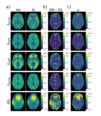
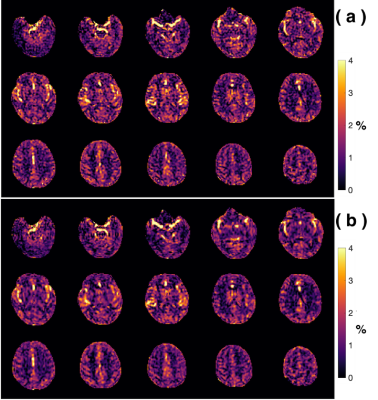
    Figure 2: DeepCEST network trained on healthy volunteers applied on a healty volunteer (a) Comparison of the predictions and the Lorentzian fit amplitudes (ground truth). (b) Error of the prediction compared to the fit. (c) Uncertainty of the prediction.
    Figure 1: a) Input data: uncorrected Z-spectra of two B1 levels acquired at 3T. b) Target data: 5-pool-Lorentzian fitted data acquired at 7T. As targets only the Lorentzian amplitudes were used.
  • Reduction of 7T CEST scan time and evaluation by L1-regularised linear projections
    Moritz Simon Fabian1, Felix Glang2, Katrin Michaela Khakzar1, Angelika Barbara Mennecke1, Alexander German1, Manuel Schmidt3, Burkhard Kasper4, Arnd Dörfler1, Frederik B. Laun1, and Moritz Zaiss1
    1Department of Neuroradiology, University Hospital Erlangen, Friedrich Alexander University Erlangen-Nürnberg, Erlangen, Germany, 2High-field Magnetic Resonance Center, Max Planck Institute for Biological Cybernetics, Tübungen, Germany, 3Department of Neuroradiology, University Hospital Erlangen, Erlangen, Germany, 4Department of Neurology, Epilepsy Center, University Hospital Erlangen, Erlangen, Germany
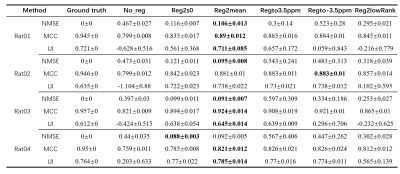
    The L1-regularized linear projection approach allows for reduction of scan time by a factor of ~2.8, while still being able to predict multiple CEST contrast parameters. It generalizes to unseen healthy subject data and tumor patient data.
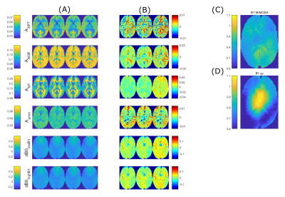
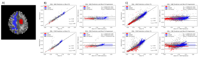
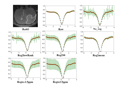
    Figure 2: Comparison of retrospective and prospective input feature reduction as well as conventional Lorentzian fitting. (A) left to right: ground truth by Lorentzian fitting on full measurement, linear prediction with all input features contained, linear prediction with retrospective reduction of input features according to the LASSO-reduced sampling schedule, measurement with these input features being prospectively omitted. (B) Difference maps of the linear predictions and the ground truth. (C) B1-MIMOSA and (D) B1-cp map as mentioned in 5
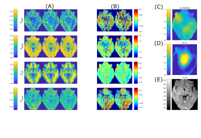
    Figure 3: Comparison of retrospective reduction of input features for a tumor patient dataset (Glioblastoma WHO grade 4). (A) left to right: ground truth obtained by Lorentzian fitting, linear prediction with all input features retained, retrospective reduction of input features. (B) Difference maps between linear predictions and ground truth. (C) B1 MIMOSA map and (D) B1-cp map as mentioned in 5. (E) Anatomical T1 contrast-enhanced image
  • Open source Pulseq interpreter for CEST MRI on Bruker systems
    Sebastian Mueller1, Kai Herz1, Klaus Scheffler1,2, and Moritz Zaiss1,3
    1High-field Magnetic Resonance Center, Max Planck Institute for Biological Cybernetics, Tuebingen, Germany, 2Department of Biomedical Magnetic Resonance, Eberhard Karls University Tuebingen, Tuebingen, Germany, 3Department of Neuroradiology, University Hospital Erlangen, Erlangen, Germany
    The proposed approach allows straightforward implementation of CEST MRI on Bruker scanners without the need of sequence programming in C. Pre-saturation is defined in open source pulseq-files which allows direct transfer to clinical devices or usage for simulations.
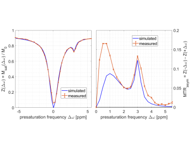
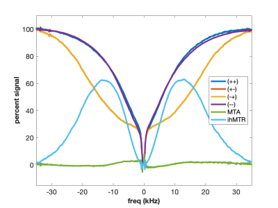
    Figure 2: Data measured (spatial mean and SD) at B0 = 14T and simulations (same pulseq-file). CEST pools included water (T1=1735ms, T2=18ms, f=100%), ssMT (T1=1000ms, T2=0.01ms, dω=0ppm, kex=23Hz, f=5%), L-arginine (T1=1000ms, T2=5ms, dω=3ppm, f=2.25%) and agar-agar (10) (T1=1000ms, T2=50ms, dω=1.6ppm, kex=6500Hz, f=1%). Details on pre-saturation and simulation source code: https://pulseq-cest.github.io/ file “APTw_3T_002”; modifications: dω list and B0. Larger deviations in MTR assymetry at <= 1.5 ppm are most likely due to residual B0 variation in the measured data.
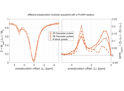
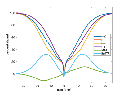
    Figure 4: (left) ROI averaged (mean ± SD) Z-spectra acquired for different CEST pres-aturation modules using Bruker’s FLASH readout. (right) MTR asymmetry.
  • Linear projection-based CEST reconstruction – the simplest explainable AI
    Felix Glang1, Moritz Fabian2, Alex German2, Katrin Khakzar2, Angelika Mennecke2, Frederik Laun3, Burkhard Kasper4, Manuel Schmidt2, Arnd Doerfler2, Klaus Scheffler1,5, and Moritz Zaiss1,2
    1High-field Magnetic Resonance Center, Max Planck Institute for Biological Cybernetics, Tübingen, Germany, 2Department of Neuroradiology, University Hospital Erlangen, Erlangen, Germany, 3Institute of Radiology, University Hospital Erlangen, Erlangen, Germany, 4Neurology, Epilepsy Center, University Clinic of Friedrich Alexander University Erlangen-Nürnberg, Erlangen, Germany, 5Department of Biomedical Magnetic Resonance, Eberhard Karls University Tübingen, Tübingen, Germany
    Linear projection-based CEST reconstruction allows mapping from acquired raw in vivo CEST data to multiple contrast parameters of interest, generalizing from healthy subject training data to unseen test data of both healthy subjects and tumor patients.
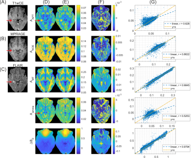
    Figure 4. Results of linear projection in a tumor patient test dataset. Clinical contrasts: (A) T1 weighted contrast-enhanced, (B) MPRAGE and (C) FLAIR. (D) Ground truth Lorentzian fit results. (E) Contrast maps obtained by linear projection with coefficients obtained from 5 healthy subject datasets. (F) Difference maps to ground truth for linear projection result. (G) Voxel-wise scatter plots of linear prediction result (y) versus ground truth (x) with legends indicating Pearson correlation coefficient r.
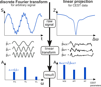
    Figure 1. Analogy of discrete Fourier transform and the proposed linear projection approach for CEST evaluation. For the Fourier transform, a signal vector S(t) is projected onto basis vectors $$$\beta_1,...,\beta_n$$$ consisting of the respective harmonics to yield the Fourier coefficients $$$A_1,...,A_n$$$ for different frequencies. For linear CEST evaluation, acquired raw data are projected onto coefficient vectors found by linear regression applied to conventionally evaluated data, to yield target contrasts like APT, NOE and ssMT amplitudes.
  • In-Vivo Sub-Minute rNOE Mapping Using AutoCEST: a Machine-Learning Approach for CEST/MT Protocol Invention and Quantitative Reconstruction
    Or Perlman1, Bo Zhu1,2, Moritz Zaiss3,4, Naoyuki Shono5, Hiroshi Nakashima5, E. Antonio Chiocca5, Matthew S. Rosen1,2, and Christian T. Farrar1
    1Athinoula A. Martinos Center for Biomedical Imaging, Department of Radiology, Massachusetts General Hospital and Harvard Medical School, Charlestown, MA, United States, 2Department of Physics, Harvard University, Cambridge, MA, United States, 3Magnetic Resonance Center, Max Planck Institute for Biological Cybernetics, Tübingen, Germany, 4Department of Neuroradiology, University Clinic Erlangen, Erlangen, Germany, 5Brigham and Women’s Hospital and Harvard Medical School, Boston, MA, United States
    A machine-learning framework was expanded for simultaneously designing the optimal CEST protocol and extracting fully quantitative maps in-vivo. A mouse tumor rNOE volume-fraction was significantly decreased, in agreement with previous human studies.
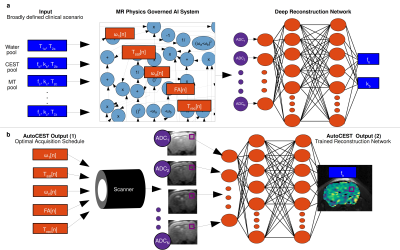
    Fig. 1 AutoCEST pipeline. a. Pre-experiment step. The broad expected range of properties (blue rectangles) are given as input to an MR physics governed AI system, which dynamically optimizes the protocol parameters (orange rectangles). The resulting “ADC” MR signals are then decoded into quantitative parameters using a deep reconstruction network. b. Experiment step. The optimal schedule parameters are loaded into the scanner, resulting in a set of N raw images. The resulting images are fed voxelwise into the trained reconstruction network, resulting in quantitative CEST maps.
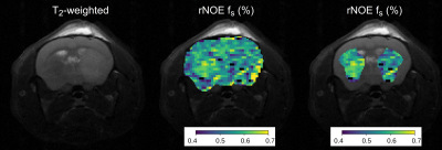
    Fig 5 In vivo study results. (Left). T2-weighted image of a tumor-bearing mouse. (Center). The corresponding rNOE volume fraction quantitative map (fs), and its overlay (right) atop the tumor and contralateral ROIs. Note the decreased fs at the tumor.
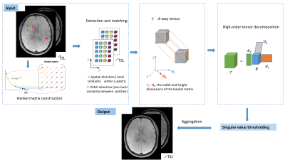
  • Whole-Brain Steady-State CEST at 3T Using MR Multitasking
    Pei Han1,2, Karandeep Cheema1,2, Hsu-Lei Lee1, Zhengwei Zhou1, Tianle Cao1,2, Sen Ma1, Nan Wang1, Anthony G. Christodoulou1,2, and Debiao Li1,2
    1Biomedical Imaging Research Institute, Cedars-Sinai Medical Center, Los Angeles, CA, United States, 2Department of Bioengineering, UCLA, Los Angeles, CA, United States
    We propose a fast 3D steady-state CEST method at 3T using MR Multitasking. By exploiting the correlation among images throughout the spatial, time, and offset frequency dimensions with a low-rank tensor, the Z-spectrum acquisition with whole-brain coverage can be done within 5.5min.
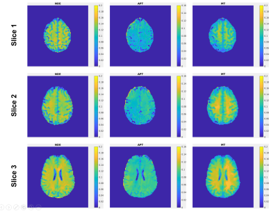
    Figure 2: Representative NOE, APT and MT maps from Multitasking ss-CEST. Three different slices are displayed to show the consistency of image quality within the 3D volume.
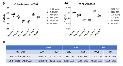
    Figure 4: Average Lorentzian amplitudes within GM and WM regions among different volunteers. The mean amplitude is consistent among healthy subjects. Contrast ratios of WM:GM for NOE/APT/MT: 1.21/1.10/1.22 (Multitasking ss-CEST) vs. 1.20/1.02/1.35 (2D single-shot FLASH CEST).
  • Deep Learning-based image reconstruction improves CEST MRI
    Shu Zhang1, Xinzeng Wang2, F. William Schuler1, R. Marc Lebel3, Mitsuharu Miyoshi4, Ersin Bayram2, Elena Vinogradov5, Jason Michael Johnson6, Jingfei Ma7, and Mark David Pagel1,7
    1Cancer Systems Imaging, MD Anderson Cancer Center, Houston, TX, United States, 2Global MR Applications & Workflow, GE Healthcare, Houston, TX, United States, 3Global MR Applications & Workflow, GE Healthcare, Calgary, AB, Canada, 4Global MR Applications & Workflow, GE Healthcare Japan, Tokyo, Japan, 5Radiology, UT Southwestern Medical Center, Dallas, TX, United States, 6Neuroradiology, MD Anderson Cancer Center, Houston, TX, United States, 7Imaging Physics, MD Anderson Cancer Center, Houston, TX, United States
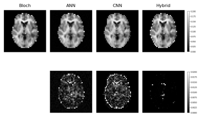
    Deep learning-based image reconstruction (DL Recon) substantially reduced the noise in the CEST maps and improved the lesion conspicuity.
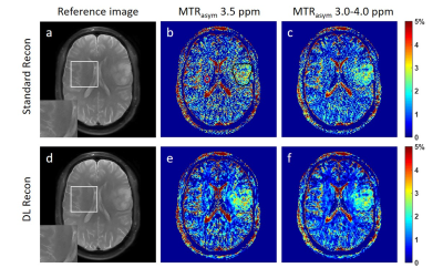
    Figure 1. The reference images using standard recon (a) and DL Recon (d). The MTRasym map at 3.5 ppm (b,e) and averaged between 3.0-4.0 ppm (c,f) using standard recon (b,c) and DL recon (e,f) of a glioma patient. The tumor ROI (black) and the background ROI of homogenous brain tissue (red) was shown in (a) as an example.
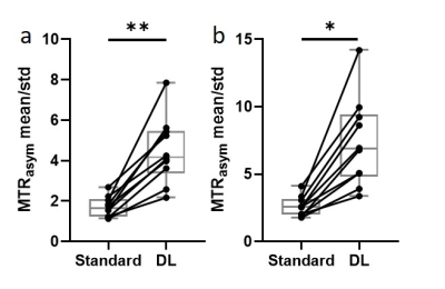
    Figure 3. The tumor ROI-averaged MTRasym divided by the standard deviation of the background ROI at 3.5 ppm (a) and 3.0-4.0 ppm (b) using standard recon and DL Recon were compared for all patients. (a) p = 0.002. (b) p = 0.016. **: p < 0.01. *: p < 0.05.
  • Indirect Inference of Acidification in Exercised Skeletal Muscle using Creatine CEST
    Dushyant Kumar1, Ryan Armbruster1, Neil Wilson2, Ravi Prakash Reddy Nanga1, and Ravinder Reddy1
    1Radiology, University of Pennsylvania, Philadelphia, PA, United States, 2Siemens Medical Solutions USA Inc, Malvern, PA, United States
    We demonstrate the feasibility of indirect detection of acidification in exercised skeletal muscle using creatine CEST findings from healthy volunteers.
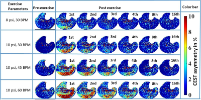
    Fig. 1: ΔCrCEST time-series for volunteer #1, corresponding to the middle slice (5th out of 8 slices). Each row corresponds to different exercise workload. Selected time frames of post-exercise CrCEST time-series are being presented, with frame number written on right top corner of each frame. The temporal resolution was 30s. Though at mild PFE level, the volunteer mostly utilized the lateral gastrocnemius (LG), both LG and medial gastrocnemius (MG) were utilized during intense PFE. As evident visually, the recovery rate increased with increased intensity of exercise levels.
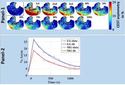
    Fig. 2: Panel -1: Time-series of Lactate CEST (LATEST) maps show intense exercise-induced changes in skeletal muscle, using images from 5th slice of volunteer #1. First LATEST frame corresponds to pre-exercise level, whereas the remaining ten frames correspond to ten time points post-exercise with 140s temporal resolution. Panel-2: Time-series plots of LATEST values averaged over the entire lateral gastrocnemius and corresponding fits are shown.
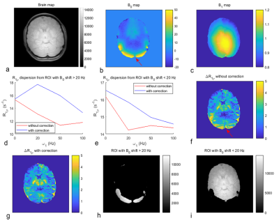
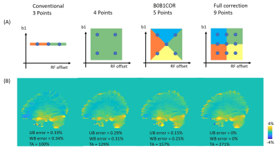
  • ­­Simultaneous mapping of B0, B1 and T1 for the correction of CEST-MRI
    Kerstin Heinecke1, Henrik Narvaez1, Christoph Kolbitsch1, and Patrick Schuenke1
    1Physikalisch-Technische Bundesanstalt (PTB), Braunschweig and Berlin, Germany
    We developed a new method for simultaneous B0-, B1- and T1- mapping, using a simple adapted CEST sequence. First results prove the feasibility of this approach and its applicability for the correction of CEST-MRI data.
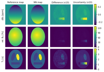
    Parameter maps and uncertainty estimation of simulated phantom data. The left column shows the reference maps with simulated B0- and B1- inhomogeneities and different brain-matter-like T1 values with 1% Gaussian noise overall and one compartment with noise ranging from 0% to 10%. From second left to right: maps generated by the NN, difference maps between reference and NN output (x10) and uncertainty maps generated by the NN (x10).
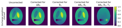
    Exchange-weighted contrasts of simulated CEST data before and after post-processing. Simulated with B0- and B1- inhomogeneities, different brain-matter-like compartments and a three-pool-system with the same CEST-pool fraction of f = 0.6% overall and one compartment with fractions ranging from 0% to 1%. Left to right: MTRRex7 contrasts of i) the uncorrected CEST-simulation and after ii) ΔB0-correction5, iii) B1-correction6, iv) ΔB0- and B1-correction. Right: AREX contrast (ΔB0-, B1- and T1-corrected)7.
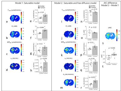
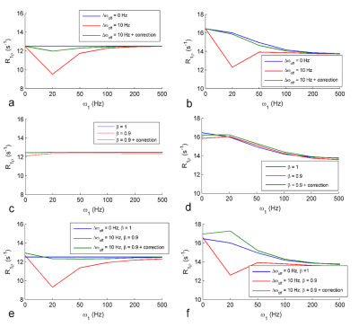
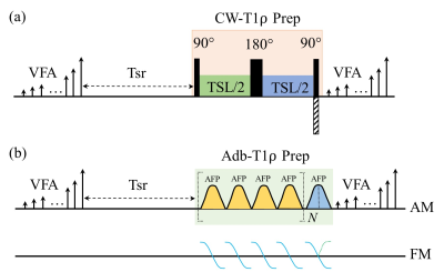
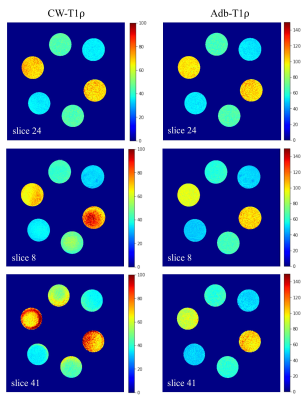
  • Quasi-steady-state (QUASS) CEST solution improves the accuracy of CEST quantification – QUASS CEST MRI-based omega plot analysis
    Phillip Zhe Sun1
    1Department of Radiology and Imaging Sciences, Emory University, Atlanta, GA, United States
    The QUASS CEST analysis accounts for the effect of finite Ts and Td and improves the accuracy of CEST MRI quantification. Both simulation and CEST MRI experiments confirmed that the QUASS solution enabled robust quantification of ksw and fr, superior over the conventional apparent CEST MRI.
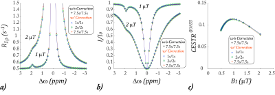
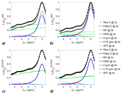
    Fig. 2., Simulation of the proposed QUASS CEST MRI. a) R1rho determined from the QUASS solution for three representative sets of Td and Ts (i.e., 1s/1s (cross markers), 2s/2s (diamond markers), and 7.5s/7.5s (plus markers) and that calculated under long Td and Ts (7.5s/7.5s, black plus markers) for B1 levels of 1 and 2 µT. b) The QUASS Z-spectra under the three representative sets of Td and Ts and two B1 levels of 1 and 2 µT. c) The QUASS CEST effect at 1.9 ppm as a function of B1 level for three sets of Ts and Td times, being 1s/1s, 2s/2s, and 7.5s/7.5s.
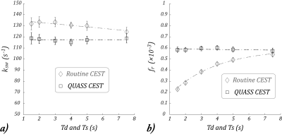
    Fig. 4., The relationship between Td/Ts with the experimentally determined ksw and fr. a) ksw from the conventional CEST MRI (circle markers) showed a significant linear dependence with Ts/Td. In comparison, ksw determined from the QUASS CEST MRI (square markers) did not show significant dependence with respect to Ts/Td. c) fr determined from conventional apparent CEST MRI (circle markers) can be described by a stretched exponential function with significant dependence on Ts/Td. d) fr determined from the QUASS CEST MRI (square markers) showed no significant dependence on Ts/Td.
  • MTC removed and exchange rate differentiated CEST using Variable Delay Multi Pulse (VDMP) in the human brain at 7T
    Bárbara Schmitz Abecassis1, Elena Vinogradov Vinogradov2,3, Jannie P. Wijnen4, Thijs van Harten1, Evita C. Wiegers4, Hans J.M. Hoogduin4, Matthias J.P. van Osch 1, and Ece Ercan1
    1Department of Radiology, Leiden University Medical Center, Leiden, Netherlands, 2Department of Radiology, UT Southwestern Medical Center, Dallas, TX, United States, 3Advanced Imaging Research Center, UT Southwestern Medical Center, Dallas, TX, United States, 4Department of Radiology, University Medical Center Utrecht, Utrecht, Netherlands
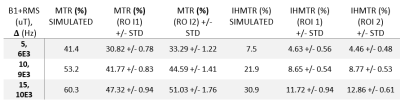
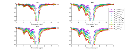
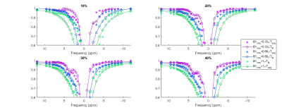
    Variable delay multi pulse (VDMP) CEST imaging at 7T allowed identifying slow and fast exchanging solute pools present in the human brain in vivo, by means of saturation build-up curves upon MTC removal and evaluation of optimal Bamplitudes.   
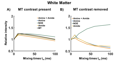
    Figure 4. A typical example of the effect of MTC on the VDMP build-up curves from the human WM for B1 = 1.99µT. In A) the saturation build-up of the different CEST-pools is plotted together with the MT contrast. In B) the MTC has been removed and the trend of the VDMP build-up curves from the CEST-pools with different exchange rates can be distinguished.
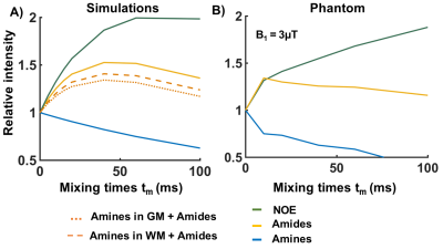
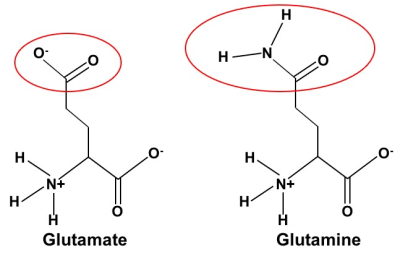
    Figure 2. Normalized VDMP saturation build-up curves for different mixing times. A) Simulated build-up curves for CEST-pools found in the human brain: according to the concentration of amines in the GM (dotted line) and WM (dashed line) B) Build-up curves from glutamate (amines in blue) and bovine serum albumin phantoms (amides in yellow and rNOE in green). Both simulation and phantom data show a gradual build-up for slow exchanging molecules (rNOE and amides) as opposed to a fast decay from fast exchanging amines.
  • Highly Accelerated 1mm3-Isotropic 3D CEST MRI with Spectral Random Walk CAIPIRINHA Sampling at 7T
    Sugil Kim1, Seong-Gi Kim2,3, and Suhyung Park4,5
    1Siemens Healthineers, Seoul, Korea, Republic of, 2Center for Neuroscience Imaging Research (CNIR), Institute for Basic Science (IBS), Suwon, Korea, Republic of, 3Department of Biomedical Engineering, Sungkyunkwan University, Suwon, Korea, Republic of, 4Department of Computer Engineering, Chonnam National University, Gwangju, Korea, Republic of, 5Department of ICT Convergence System Engineering, Chonnam National University, Gwangju, Korea, Republic of
    We propose highly accelerated 3D CEST MRI using CAIPI sampling based 3D segmented EPI with spectral random walk, potentially enabling 1mm-isotropic whole-brain CEST imaging within 5min at 7T.
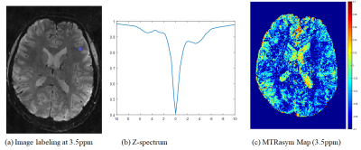
    Fig3 (a) CEST labeling image at 3.5ppm, (b) Z-spectrum with marked as blue circle in (a), and (c) MTR asymmetric map at 3.5ppm.
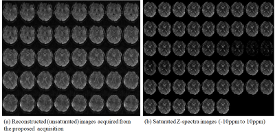
    Fig2 (a) Reconstructed (unsaturated) images acquired from the proposed acquisition, (b) Saturated Z-spectra images offset frequencies -10ppm to 10ppm
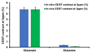
  • Mapping of intracellular pH in vivo using amide and guanidyl CEST-MRI at 9.4 T
    Philip S Boyd1, Johannes Breitling1, Stephanie Laier2, Karin Mueller-Decker2, Andrey Glinka3, Mark E Ladd1, Peter Bachert1, and Steffen Goerke1
    1Division of Medical Physics in Radiology, German Cancer Research Center (DKFZ), Heidelberg, Germany, 2Center for Preclinial Research, Core Facility Tumor Models, German Cancer Research Center (DKFZ), Heidelberg, Germany, 3Division of Molecular Embryology, German Cancer Research Center (DKFZ), Heidelberg, Germany
    The presented method allows calculation of reliable pH maps in the presence of varying concentration, superimposing CEST signals, magnetization transfer and spillover dilution. Applicability in vivo was demonstrated in mice showing an average intracellular pH in tumors of approximately 7.
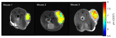
    Figure 3: In vivo application of the calibrated pH-CEST technique in tumor-bearing mice. pH values of 6.97 ± 0.09, 7.00 ± 0.20 and 7.13 ± 0.19 were found in the subcutaneous lesions of three DLD xenografted nude mice.
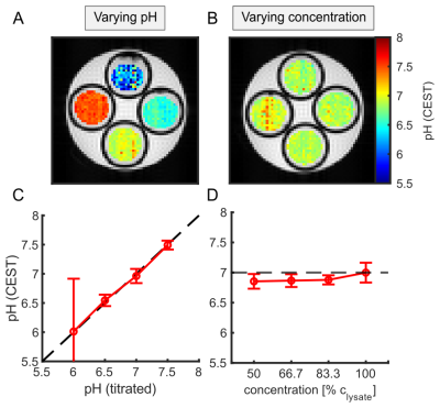
    Figure 2: Correlation of calculated pH from CEST-MRI with titrated pH (A,C) and tissue concentration (B,D) of porcine brain lysate. C: Correlation of the titrated pH and the mean pH values calculated from the CESTratio. D: Mean pH values calculated from the CESTratio as a function of concentration.
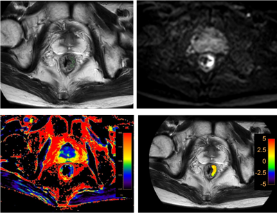
  • 7 tricks for 7T CEST: improving the reproducibility of multi-pool evaluation
    Angelika Mennecke1, Katrin Khakzar1, Kai Herz2, Moritz Fabian1, Alexander German1, Andrzej Liebert3, Ingmar Blümcke4, Burkhard Kasper5, Manuel Schmidt1, Arnd Dörfler1, Armin Nagel3, Frederik Laun3, and Moritz Zaiß1
    1Department of Neuroradiology, University Hospital of Erlangen, FAU Erlangen-Nürnberg, Erlangen, Germany, 2High-field Magnetic Resonance Center, Max Planck Institute for Biological Cybernetics, Tübingen, Germany, 3Institute of Radiology, University Hospital of Erlangen, FAU Erlangen-Nürnberg, Erlangen, Germany, 4Institute of Neuropathology, University Hospital of Erlangen, FAU Erlangen-Nürnberg, Erlangen, Germany, 5Department of Neurology, Epilepsy Centre, University Hospital of Erlangen, FAU Erlangen-Nürnberg, Erlangen, Germany
    With the help of the presented post-processing procedure, it is possible to obtain an increased reproducibility. For the amide contrast, the CoV decreased from 4% to less than 1.2 %.
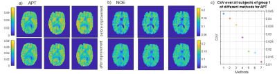
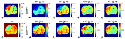
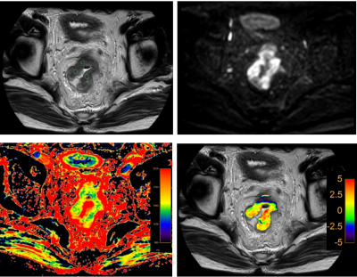
    a) APT maps and b) NOE maps of a repeated measurement (group 1) before and after improving the post-processing steps (colorbar adjusted for visual comparison) c) decreasing CoV as a function of the stepwise improvement of post-processing methods: 1) moco with interpolation, 2) additionally, 2 point M0 normalization, 3) moco to the offset at 3.5 ppm, 4) B0 correction by using a Lorentzian fit 5) B0 correction with spline interpolation parameter 0.999 6) 2 point MZ normalization 7) LFM 4
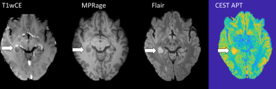
    Conventional images (contrast-enhanced T1 weighted imaging, MPRage, and Flair) and CEST APT image of an epilepsy-associated tumor initially diagnosed as low grade, histologically proven to be glioblastoma, IDH wild-type. Improved CEST postprocessing pipeline was used.
  • Pulseq-CEST: Towards multi-site multi-vendor compatibility and reproducibility of CEST experiments using an open source sequence standard
    Kai Herz1,2, Sebastian Mueller1, Maxim Zaitsev3, Linda Knutsson4,5, Jinyuan Zhou5, Phillip Zhe Sun6, Peter van Zijl5,7, Klaus Scheffler1,2, and Moritz Zaiss1,8
    1Magnetic Resonance Center, MPI for Biological Cybernetics, Tuebingen, Germany, 2Biomedical Magnetic Resonance, University of Tuebingen, Tuebingen, Germany, 3Center for Medical Physics and Biomedical Engineering, Medical University of Vienna, Vienna, Austria, 4Medical Radiation Physics, Lund University, Lund, Sweden, 5Russell H. Morgan Department of Radiology and Radiological Science, Johns Hopkins University School of Medicine, Baltimore, MD, United States, 6Yerkes Imaging Center, Emory University, Atlanta, GA, United States, 7F.M. Kirby Research Center for Functional Brain Imaging, Kennedy Krieger Institute, Baltimore, MD, United States, 8Neuroradiology, Friedrich‐Alexander Universität Erlangen‐Nuernberg, Erlangen, Germany
    Pulseq-CEST enables a straightforward approach to standardize, share, simulate and measure different CEST preparation schemes, which are inherently completely defined.
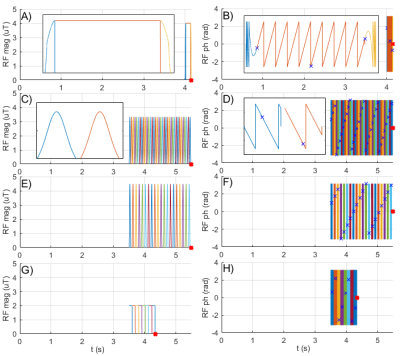
    RF magnitude A) and phase B) of the spin-lock saturation at 0.6 ppm. The frequency modulation can be seen from the changing phase in the zoomed plot (black rectangle). The red dot marks the beginning of the readout period. RF magnitude (C,E,G) and phase (D,F,H) during three different APTw protocols: APTw_3T_001 (C,D), APTw_3T_002 (E,F) and APTw_3T_003 (G, H) all with B1,cwpe = 2 µT and recovery time, Trec = 3.5 s. In C) and D), a zoomed graph for two RF pulses is shown in the black rectangles. The phase accumulation due to the off-resonance of the RF pulses is taken into account (D).
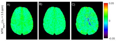
    MTRasym maps at 3.5 ppm for the APTw_3T_001 (A), APTw_3T_002 (B) and APTw_3T_003 (C) protocols. Protocols were run with repeated acquisitions (3 repetitions) at the offsets of interest and a dummy scan at the beginning.
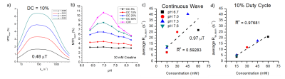
  • Assessment of acquisition strategies of CEST MR fingerprinting pH imaging using Cramer-Rao Bound algorithm
    Jie Liu1, Hui Liu2, Qi Liu2, Jian Xu2, Hairong Zheng1, and Yin Wu1
    1Paul C. Lauterbur Research Center for Biomedical Imaging, Shenzhen Institutes of Advanced Technology, Chinese Academy of Sciences, Shenzhen, China, 2United Imaging Healthcare America, Houston, TX, United States

    We designed a Cramer-Rao bound based metric, and demonstrated its ability in evaluating the performance of acquisition strategies of CEST-MRF imaging in pH quantification. 

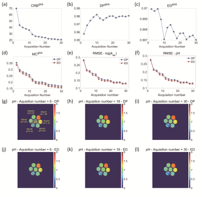
    Figure 3. (a-c) Values of CRB-, DP-, ED-based indexes with varied acquisition number of 2-30; (d) RMSE of pH in MC simulation study using both DP- and ED-based matching methods; RMSE of (e) log(kex) and (f) respective pH values of the phantoms; the CEST-MRF measured pH maps in the phantom study using both (g-i) DP- and (j-l) ED-based matching methods for representative acquisition numbers of (g, j) 6, (h, k) 18 and (i, l) 30.
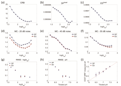
    Figure 1. (a-c) Alterations of CRB-, DP-, ED-based metrics with exchange rates; RMSE of pH quantification in MC simulation study using both DP- and ED-based matching methods under noise levels of (d )20, (e) 40 and (f) 55 dB; RMSE of (g) log(kex) and (h) pH of the phantom; (i) correlation of the measured and the titrated pH values for vials with the same concentration of 60mM.
  • A comparison of several tumor endogenous pH mapping methods using CEST at 11.7T
    Ying Liu1,2, Botao Zhao1,2, and Xiao-Yong Zhang1,2
    1Institute of Science and Technology for Brain-Inspired Intelligence, Fudan University, Shanghai, China, 2Key Laboratory of Computational Neuroscience and Brain-Inspired Intelligence (Fudan University), Ministry of Education, Shanghai, China
    We compared several tumor endogenous pH mapping methods using CEST at 11.7T. All of these pH-weighted contrasts showed a pH correlation, while the pH enhanced and APT methods were not concentration-independent and the sensitivity of AACID was affected by the weak amine signals at 2.7ppm.
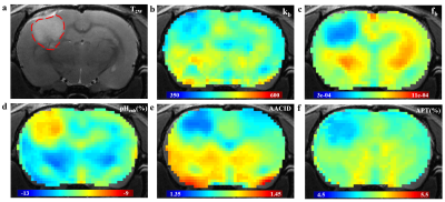
    Fig. 2. Representative examples of structural image and CEST maps of one mouse brain. (a)T2W image with tumor region delineated by the red dotted line. (b), (c) Representative proton exchange rate and labile proton ratio maps. (d), (e), (f) pH weighted contrasts calculated using pH enhanced method, AACID method and amide proton transfer (APT) MRI.
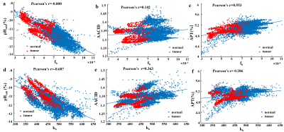
    Fig. 3. Association between labile proton ratio (fb) , chemical exchange rate (kb) values and AACID (a) (d) ,pHenh (b) (e), APT(c) (f) values of all voxels in 6 mice brain from tumors (red points) and normal tissue (blue points).
  • Whole-brain amide CEST at 3T with a steady-state radial MRI acquisition
    Ran Sui1,2,3, Lin Chen1,2, Yuguo Li1,2, Jianpan Huang4, Kannie W.Y Chan2,4, Xiang Xu5, Peter C.M.van Zijl1,2, and Jiadi Xu1,2
    1F.M. Kirby Research Center for Functional Brain Imagin, Kennedy Krieger Institute, Baltimore, MD, United States, 2Russell H. Morgan Department of Radiology and Radiological Science, Johns Hopkins University School of Medicine, Baltimore, MD, United States, 3Department of Biomedical Engineering, Johns Hopkins University, Baltimore, MD, United States, 4Department of Biomedical Engineering, City University of Hong Kong, Hong Kong, China, 5BioMedical Engineering and Imaging Institute, Icahn School of Medicine at Mount Sinai, New York, NY, United States
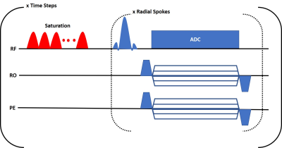
    Acquire whole-brain amide CEST mapping at 3T MRI by using steady-state radial sampling CEST with PROPELLOR-based sampling
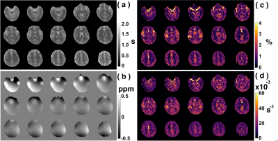
    Figure 3: Typical multi-slice human brain images acquired with starCEST at 3T. (a) T1 maps by look-locker sequence; (b) B0 maps acquired with dual-echo sequence, The (c) amideCEST maps (ΔZamide) and the corresponding (d) apparent relaxation rate (Ramide) maps extracted with the PLOF method by including the B0 and T1 maps, respectively.
    Comparison of the amideCEST maps without and with MLSVD post-processing. (a) The original amide CEST maps extracted using PLOF without MLSVD denoising. (b) MLSVD denoising applied with truncation numbers 48, 48 and 10.
  • Investigating MT and CEST Characteristics of DU145 Prostate Tumour Xenografts in Relation to Radiation Treatment Response
    Leedan Murray1, Wilfred W. Lam1, and Greg J. Stanisz1,2
    1Physical Sciences, Sunnybrook Research Institute, Toronto, ON, Canada, 2University of Toronto, Toronto, ON, Canada
    MT and CEST characteristics of DU145 prostate tumour xenografts with known responses to radiation were investigated. Significant changes between responses were mostly observed in the necrotic/apoptotic regions of the tumour and were most evident in the qMT parameters.
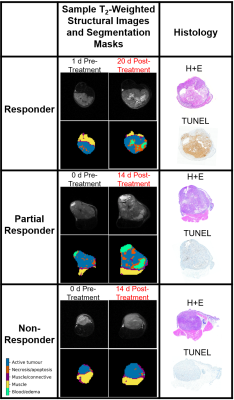
    Figure 1: Representative segmentation masks, T2-weighted images and histology (H+E and TUNEL stains) for each category of response to radiation treatment (responder, partial responder, non-responder).
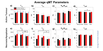
    Figure 4: Average estimated qMT parameters by treatment response of (a-d) active and (e-h) necrotic/apoptotic regions. Free parameters were: T1 and T2 of the water pool (T1,L and T2,L respectively), the exchange rate of magnetization from the MT pool to the water pool (RMT), original magnetization of the MT pool relative to the water pool (M0,MT), and T2 of the MT pool (T2,MT). *p < 0.05. **p < 0.01.
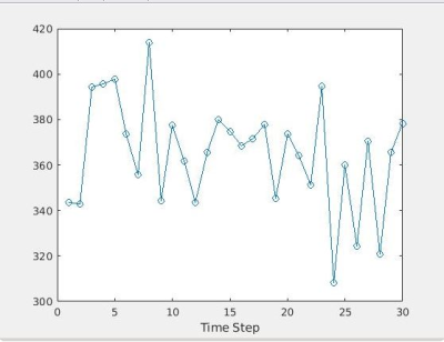
  • An ASL and CrCEST combined protocol at 3T in the Study of Metabolic and Perfusion Changes Post Revascularization in Peripheral Arterial Disease
    Helen Sporkin1, Toral Patel2, Christopher Schumann2, Christopher Kramer2,3, and Craig Meyer1,3
    1Biomedical Engineering, University of Virginia, Charlottesville, VA, United States, 2Cardiovascular Medicine, University of Virginia, Charlottesville, VA, United States, 3Radiology and Medical Imaging, University of Virginia, Charlottesville, VA, United States
    Our preliminary findings in six patients show success in imaging PAD patients with CrCEST and exercise-induced hyperemia ASL in the same protocol. Further recruitment is necessary to establish findings linking perfusion, metabolism, and function. 
    Figure 1: (Top row) CrCEST time course imaging (left) ,and ASL (middle), and overall CrCEST decay (right) in a patient with an ABI of 0.68 prior to endovascular revascularization.(Bottom row) CrCEST time course imaging (left) , ASL (middle), and overall CrCEST decay (right) CrCEST time course imaging and ASL in the same patient 6 months after revascularization, showing changes in both metabolism and perfusion.
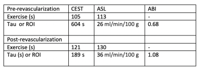
    Table 1: CEST and ASL evaluation pre and post revascularization in patient 1. ASL and CEST measurements are reported as a mean of the muscle ROI in which the greatest perfusion was seen in the ASL images.
Back to Top
Digital Poster Session - T1ρ, MT & CEST
Contrast Mechanisms
Monday, 17 May 2021 17:00 - 18:00
  • Accelerating T1ρ mapping using patch-based low-rank tensor
    Yuanyuan Liu1, Zhuo-Xu Cui1, Xin Liu1, Dong Liang1, and Yanjie Zhu1
    1Shenzhen Institutes of Advanced Technology, Chinese Academy of Sciences, Shenzhen, China
    The proposed method offers better performance than the existing methods in retrospective experiments and can significantly reduce the scan time of T mapping. This technique might help facilitate fast T mapping in clinics.
    Figure 1. The flow diagram of the proposed method PLANT.
    The T1ρ-weighted images at TSL=1ms reconstructed using PLANT, HD-PROST and L+S with different acceleration factors (R=4, 5 and 6) from retrospectively undersampled data. The corresponding error maps are also shown for comparison. The reference image is obtained from the fully sampled k-space data.
  • Robust Quantitative T1rho imaging
    Huimin Zhang1, Baiyan Jiang1, Jian Hou1, Queenie Chan2, and Weitian Chen1
    1Imaging and Interventional Radiology, The Chinese University of Hong Kong, Sha Tin, Hong Kong, 2Philips Healthcare, Hong Kong, Hong Kong
    We utilized AC-iTIP and combined it with a proposed correction method to achieve robust quantification of T1rho.
    Figure 3. a) A raw image acquired using AC-iTIP at TSL 0 ms. b) The fitting results from the selected ROI in a). c) The ground-truth T1rho map acquired. d) and e) show the T1rho map before and after correction, respectively. f) compares the T1rho values in c)-e). Blue, red and yellows bars represent c), d) and e), respectively.
    Figure 4. a)-c) and d)-e) show B1 and B0 field maps from three different scans. g)-i) and j)-l) show the T1rho maps in vivo before and after correction. The cartilage and muscle are manually drawn for analysis.
  • R1ρ Dispersion imaging in human skeletal muscle at 3 Tesla
    Fatemeh Adelnia1, Zhongliang Zu1,2, Feng Wang1,2, Kevin D Harkins3, and John C Gore1,2,3,4,5
    1Vanderbilt University Institute of Imaging Science, Nashville, TN, United States, 2Department of Radiology and Radiological Sciences, Vanderbilt University Medical Center, Nashville, TN, United States, 3Department of Biomedical Engineering, Vanderbilt University, Nashville, TN, United States, 4Department of Physics and Astronomy, Vanderbilt University, Nashville, TN, United States, 5Department of Molecular Physiology and Biophysics, Vanderbilt University, Nashville, TN, United States
    R dispersion over a range of weak locking fields has the potential to reveal information on microvascular geometry and density. This work presents in-vivo results supporting the application of this technique to the measurement of microvascular sizes and spacings in skeletal muscle. 
    Fig 1. a) Schematic diagram of an imaging voxel illustrating the chemical exchange of labile hydrogen, between water and hydroxyls, occurring in the presence of susceptibility gradients generated by the red blood cells containing paramagnetic deoxyhemoglobin. b) Simulated R dispersions for a spherical structure with a radius of 10 μm. The low-frequency dispersion corresponds to diffusion effects (blue), the high frequency corresponds to exchange (red), and the composite curve “double dispersion” added two rates linearly R = Rdipolar + RDiff + REx (adapted from Ref 3).
    Fig 5. 3D T images collected with the anterior coil, Slice N=3, TR = 1250 ms, shortest TE, SENSE factor 2, a FOV of 224 x 224 mm, and a voxel size of 1 x1 x 8 mm with TSL; 2, 12, 36 ms and FSL=0, 60, 120, 200, 300, 480 Hz resulted in a total scan time of 7 min and 56 sec. (a) Example of anatomy and R=1/T maps from slice #3. ROI placed in the area that has approximately B0 off-set less than 30Hz. (b) Averaged R values from selected ROI. The error bars show the standard deviation. The fitted curve calculated using R equation (c) Fitted parameters extracted from R dispersion depicted in (b).
  • Highly accelerated T1ρ imaging using kernel-based low-rank compressed sensing reconstruction in knees with and without osteoarthritis
    Jeehun Kim1,2, Chaoyi Zhang3, Mingrui Yang1, Hongyu Li3, Mei Li1, Richard Lartey1, Leslie Ying3,4, and Xiaojuan Li1
    1Department of Biomedical Engineering, Program of Advanced Musculoskeletal Imaging (PAMI), Cleveland Clinic, Cleveland, OH, United States, 2Department of Electrical Engineering, Case Western Reserve University, Cleveland, OH, United States, 3Electrical Engineering, University at Buffalo, State University of New York, Buffalo, NY, United States, 4Biomedical Engineering, University at Buffalo, State University of New York, Buffalo, NY, United States
    Compared to reference images, cartilage T coefficients of variation < 3.5% was achieved with prospective acceleration factor of 8, which reduced the scan time to 3 minutes, for subjects with and without osteoarthritis.
    Figure 4 Sample images of reference and accelerated T map. The T map of cartilage compartments was overlaid to the corresponding DESS images for better visualization.
    Figure 3 (a) shows the CV between reference and accelerated T value, scan-rescan CV, and scan-rescan ICC with a 95% confidence interval. (b) shows the Bland-Altman plot between accelerated and reference T value. Each entry corresponds to an average value of a cartilage compartment in a subject. ICC was calculated for each AF.
  • Reproducible high-resolution T1ρ maps of the brain in under seven minutes using compressed sensing
    Gabriele Bonanno1,2,3, Tom Hilbert4,5,6, Patrick Leibig7, and Tobias Kober4,5,6
    1Advanced Clinical Imaging Technology,Siemens Healthcare AG, Bern, Switzerland, 2Translational Imaging Center, sitem-insel AG, Bern, Switzerland, 3Departments of Radiology and Biomedical Research, University of Bern, Bern, Switzerland, 4Advanced Clinical Imaging Technology, Siemens Healthcare AG, Lausanne, Switzerland, 5Department of Radiology, University Hospital (CHUV) and University of Lausanne (UNIL), Lausanne, Switzerland, 6LTS5, École Polytechnique Fédérale de Lausanne, Lausanne, Switzerland, 7Siemens Healthcare GmbH, Erlangen, Germany
    High isotropic resolution and full-brain T1ρ maps obtained at the scanner from an accelerated and optimized FLASH sequence are demonstrated to provide high repeatability and reproducibility in a healthy volunteer cohort.

    Figure 3

    Representative T-prepared images (only SL-time=30 ms shown in top row) and T map (bottom row) obtained from the same acquisition. Homogenous T contrast can be observed in the whole brain, even in lower structures for SL-time=30 ms. Occasionally some artifacts may be observed above the nasal cavity due to air-tissue boundaries (arrow). Quantification of T also shows good contrast and homogeneity throughout the brain.

    Figure 4

    Example sagittal slices from T-prepared volumes and the resulting map in the same subject during Reference, Repeat and One-Week scan show increased T weighting as function of SL-time as well as good visual repeatability and reproducibility of image quality between scans.

  • Correction of errors in estimates of T1ρ at low spin-lock amplitudes in the presence of B0 and B1 inhomogeneities
    Zhongliang Zu1, Fatemeh Adelnia1, Kevin Harkins1, Feng Wang1, and John Gore1
    1Vanderbilt University Medical Center, Nashville, TN, United States
    Spin-lock imaging at low locking amplitudes may provide information on tissue microvasculature. But there are residual errors in estimates of R1ρ even if composite pulse preparations are used. In this work, we developed an approximate theoretical analysis to correct these errors.
    FIG.3 Maps of brain (a), B0 (b), B1 (c), and ΔR (the subtraction of two R maps acquired with ω1 of 0 and 100Hz), without/with correction (f, g) from a healthy human subject. (d, e) show the averaged R dispersions without/with correction from the ROI with large B0 shift (│Δωoff│ > 20 Hz) (h) and small B0 shift (│Δωoff│ < 20 Hz) (i), respectively.
    FIG. 2. Single-pool (a, c, e) and two-pool (b, d, f) model simulated R dispersions under B0 shift (a, b), B1 shift (c, d), and both B0 and B1 shift (e, f), and with correction (green lines) and without correction (red lines). R dispersions with no shifts in either B0 or B1 (blue lines) were also plotted for comparison. Simulation parameters included T1a=1.5s, T2a=80ms, T1b=1s, T2b=30ms; fractional concentration of pool B is 0.2; the exchange rate from pool B to pool A is 20s-1; resonance frequency of pool A is 0 Hz and pool B is 63.5 Hz.
  • High Resolution Adiabatic T1ρ Mapping Using 3D MAPSS Sequence at 3T
    Can Wu1,2 and Qi Peng3
    1Department of Medical Physics, Memorial Sloan Kettering Cancer Center, New York, NY, United States, 2Philips Healthcare, Andover, MA, United States, 3Department of Radiology, Albert Einstein College of Medicine and Montefiore Medical Center, Bronx, NY, United States
    3D MAPSS T1ρ mapping with adiabatic RF pulses is less sensitive to frequency offset compared to conventional 3D MAPSS T1ρ mapping with continuous-wave RF pulses, potentially leading to more accurate T1ρ quantification in the presence of field inhomogeneities.
    Figure 1. (a). CW-T1ρ preparation is implemented by a composite RF pulse (90°-TSL/2-180°-TSL/2-90°). Phase cycling of CW-T1ρ is achieved by a phase reversal of the last 90° pulse. (b). Adb-T1ρ is achieved by a series of four adiabatic full passage (AFP) pulse group following MLEV phase cycling. The frequency modulation of the second half of the last AFP pulse is reversed for phase cycling. N: number of repeats of the four AFP pulse group; VFA: variable flip angle; TSL: time of spin lock, Tsr: time for saturation recovery. AM: amplitude modulation; FM: frequency modulation.
    Figure 2. Example phantom T1ρ maps from 3D MAPSS CW-T1ρ (left) and Adb-T1ρ (right) at the center slice 24 (top row), off-center slice 8 (middle row) and off-center slice 41 (bottom row). Slice 8 and slice 41 of CW-T1ρ clearly show non-uniform T1ρ maps due to artifacts from frequency offset, while the T1ρ maps from Adb-T1ρ are more uniform and consistent at the two off-center slices. CW-T1ρ: continuous-wave T1ρ mapping; Adb-T1ρ: adiabatic T1ρ mapping.
  • Comprehensive T1ρ Measurement of in vivo Lumbar Intervertebral Discs using a 3D Adiabatic T1ρ Prepared UTE (UTE-Adiab-T1ρ) Sequence
    Zhao Wei1,2,3, Alecio F. Lombardi1, Zubiad Ibrahim1, Mohammadamin Cheraghi1, Koihi Masuda4, Jiang Du1, Eric Y. Chang1,5, Graeme M. Bydder1, Wenhui Yang2,3, and Ya-Jun Ma1
    1Department of Radiology, UC San Diego, San Diego, CA, United States, 2Institute of Electrical Engineering, Chinese Academy of Sciences, Beijing, China, 3University of Chinese Academy of Sciences, Beijing, China, 4Department of Orthopedic Surgery, UC San Diego, San Diego, CA, United States, 5Radiology Service, Veterans Affairs, San Diego Healthcare System, San Diego, CA, United States
    The UTE-Adiab-T technique can quantify the T of whole lumbar IVDs, including the nucleus pulposus, annulus fibrosis and cartilaginous endplate. This may be valuable for comprehensive assessment of IVD degeneration.
    Figure 2. Representative T maps (first row) and corresponding T2w-FSE images (second row) of four subjects (as shown in four columns respectively). These T maps demonstrate that UTE-Adiab-T sequence allows measurement of Ts of the whole IVD, including the CEP. In comparison, the CEP regions were low signal on the T2w-FSE images. The modified Pfirrmann grades of discs are included on the T2w-FSE images.
    Figure 3. Spearman’s correlation coefficient results between modified Pfirrmann grades and T values of OPAF (a), SCEP (b), ICEP (c), and NP (d). A strong negative correlation is observed in the NP, and moderate positive correlations are observed in the OPAF, SCEP, and ICEP.
  • Quantitative inhomogeneous MT with Cramer Rao lower bound optimized protocol to distinguish tissue from donors with/without Multiple Sclerosis
    Gopal Varma1, Aaron K Grant1, Olivier M Girard2, Guillaume Duhamel2, and David C Alsop1
    1Radiology, Division of MR Research, Beth Israel Deaconess Medical Center, Harvard Medical School, Boston, MA, United States, 2CNRS, CRMBM, Aix-Marseille Univ, Marseille, France
    Quantitative inhomogeneous Magnetization Transfer of brain and spinal cord tissues showed differences in free pool longitudinal relaxation rate R1a, bound pool transverse relaxation time T2b, and dipolar relaxation time T1d between samples from donors with and without multiple sclerosis.
    Figure 4 IhMT images and maps of selected qihMT parameters output from global fits to ihMT data acquired with optimized protocol in central nervous system tissue from donors with and without MS. The ihMT images in the top row are formed from the difference between the summation of data prepared with single or dual frequency RF irradiation applied off-resonance. Color bars on the right relate to the maps of qihMT parameters in the same row all with lowest levels of 0 and highest indicated. All images and maps were resized to twice their resolution by nearest-neighbor interpolation.
    Figure 1 Schematic of MT sequence (top) for ihMT experiments illustrating some of the scan parameters open to optimization and table of optimal protocol of scan parameters (bottom) from CRLB analysis. Optimized parameters included: MT preparation duration (𝛕RF), recovery time (𝛕rec), root mean square B1 (B1,RMS) over the MT preparation, and frequency (𝛥), pulse width (pw), and duty cycle (DC) of MT pulses.
  • Fast 3D steady state inhomogeneous magnetization transfer imaging with Segmented Spoiled Gradient Echo - Echo Planar Imaging.
    Masanori Ozaki1 and Masao Yui1
    1Research and Development Center, Canon Medical Systems Corporation, Kawasaki, Japan
    Inhomogeneous magnetization transfer can produce myelin-specific contrast, however long acquisition times are necessary for acquisitions with whole-brain coverage. Our proposed method achieved reduced acquisition times without SNR penalty compared to previous reports.
    Figure 2. Representative maps of: a,c) ihMTR; b,d) ihMTRinv; a,b) maps calculated by 3D segmented SPGR dataset and c,d) maps calculated by 3D segmented SPGR-EPI dataset from a healthy volunteer, as acquired in the sagittal plane, and reformatted into the coronal and axial planes.
    Figure 1. Sequence diagrams used to acquire data for: a) ihMT, and b) reference using a T1 preparation.
  • Accelerated Fitting for Quantitative Magnetization Transfer in Glioblastoma Multiforme Patients with Uncertainty using Deep Learning
    Matt Hemsley1,2, Rachel W Chan2, Liam Lawrence1,2, Sten Myrehaug3,4, Arjun Sahgal2,3,4, and Angus Z Lau1,2
    1Medical Biophysics, University of Toronto, Toronto, ON, Canada, 2Department of Physical Sciences, Sunnybrook Research Institute, Toronto, ON, Canada, 3Department of Radiation Oncology, Sunnybrook Health Sciences Centre, Toronto, ON, Canada, 4Department of Radiation Oncology, University of Toronto, Toronto, ON, Canada
    Neural network models were compared to a non-linear least squares fitting of the Bloch-McConnell equations for reconstruction of quantitative magnetization transfer images. Runtime was reduced from 10 hours/slice to 1 second/slice with approximately 1% error.
    Fig 2. Example M0b outputs. The first column shows the output of the non-linear least-squares fit of the Bloch McConnell equations used as the ground truth. Subsequent columns show the ANN, CNN, and Hybrid model outputs. The second row contains the difference maps of the associated model and Bloch-McConnell fit.
    Fig 3. Model performance. A) Example segmentation of GTV and cNAWM. B) and C) show Bland Altman plots of the single slice in A, and the full test set, respectively. Scatterplots show the relationship between network predictions and the non-linear least-squares fit of the Bloch-McConnell equations, and the Pearson correlation coefficient for each ROI. The difference plots evaluate the bias (solid line, dashed lines 95% CI) between mean differences of the network and ground truth in each ROI.
  • Super-Lorentzians and MT Asymmetries and Dipolar Order – Oh My!
    Scott D. Swanson1
    1Department of Radiology, University of Michigan, Ann Arbor, MI, United States
    MT studies of model systems controlling MT asymmetry and ihMTR.
    Figure 4. MT studies of CA:SD:BTAC. MT is generated by exchange of water protons with amide protons of SD and hydroxyl protons of CA. MTA is relatively small as the two exchange mechanisms balance. Note that the red line of the figure, (+-) RF saturation, is not visible as the yellow line, (-+) RF saturation, is identical and overwrites the (+-) line. T1d in this sample is long and eMT is much larger that conventional MT. This leads to a large ihMT signal.
    Figure 6. MT studies of CA:SD:BTAC plus cholesterol. Cholesterol provides an additional hydroxyl proton for cross-relaxation and a different underlying chemical shift profile. Addition of rigid cholesterol increases MTA relative to pure CA:SD:BTAC shown in Fig. 4. The MT asymmetry of cholesterol is also very broad. ihMTR is decreased as cholesterol stiffens the membrane and decreases proton T1d times, allowing for more efficient intermolecular spin diffusion in the lipid matrix.
  • Toward more specific imaging of fibrosis: The z-spectrum of collagen
    Nabeelah Jinnah1, Olivier Mougin1, Penny Gowland1, Caroline Hoad1, Gordon Moran1, Andrew Carradus1, and Hannah Williams1
    1University of Nottingham, Nottingham, United Kingdom
    Collagen is an important contribution to tissue fibrosis. We have characterized the z-spectrum of collagen in phantoms at 3T and 7T. We found two peaks at +1.9 ppm and +3.5 ppm. Fitting to the Bloch McConnell equations using a PSO algorithm yielded pool sizes that increased with concentration.
    Figure 2: Spectra acquired at 7T at 5 different powers and fitted using the PSO algorithm, with an acquisition time of 9s/frequency.
    Figure 1: Spectra acquired at 3T for the diverse concentration and at 3 different saturation powers and fitted using the PSO algorithm, with an acquisition time of 21s per frequency.
  • Differential diagnosis rectal cancer with and without lymph node metastasis using amide proton transfer-weighted imaging and T1 map
    Anliang Chen1, Ailian Liu1, Jiazheng Wang2, Zhiwei Shen2, Deshuo Dong1, Wan Dong1, Yuhui Liu1, Qingwei Song1, and Renwang Pu1
    1Radiology, The First Affiliated Hospital of Dalian Medical University, Dalian, China, 2Philips Healthcare, Beijing, China
    APTw imaging combined with T1 map can effectively reflect lesion changes between rectal cancer with and without lymph node metastasis.
    Figure 1. A 65-year-old male patient with lymph node metastasis of rectal cancer. T2W image (a), DWI (b), T1 map (c), and APTw-T2W fusion image (d) to show the lesion of rectal cancer with lymph node metastasis. Three ROI of rectal cancer were showed on T2W image. APT and T1 values of the ROI were 0.89%, 0.45%, 0.97% and 1579.90ms, 1449.80ms, 1496.05ms.
    Figure 2. A 64-year-old male patient without lymph node metastasis of rectal cancer. T2W image (a), DWI (b), T1 map (c), and APTw-T2W fusion image (d) to show the lesion of rectal cancer without lymph node metastasis. Three ROI of rectal cancer were showed on T2W image. APT and T1 values of the ROI were 2.03%, 2.64%, 1.73% and 1371.23ms, 1337.87ms, 1353.56ms.
  • B0 and B1 correction anti-respectively for chemical exchange saturation transfer imaging
    Ying-Hua Chu1, Yi-Cheng Hsu1, and Patrick Alexander Liebig2
    1MR Collaboration, Siemens Healthcare Ltd., Shanghai, China, 2Siemens Healthcare GmbH, Erlangen, Germany
    We proposed a new B0/B1 correction method that undersamples the number of offsets. For APTw imaging in brain, the method halved the error caused by B1 inhomogeneity at 3T with 157% scan time.
    Figure2: (A) The illustration of B1 and RF offsets sampling and correction methods for conventional, 4 points, B0B1CAR, and full correction methods, respective. (B) The sagittal APTw images with B0 and B1 correction by the corresponding methods. The mean errors in the upper brain region (UB error) and the whole brain region (WB error) are measured by the mean difference[LP(DMRS1] with the full correction method. The relative total acquisition times (TA) are compared with the conventional method.
    Figure1: (A) Conventional method for CEST B0 and B1 correction. First, the data at the targeted z-spectrum frequency was interpolated at each B1 value. Then, the data at the targeted frequency and B1 were interpolated from the B0 corrected data. (B) B0B1COR method for CEST B0 and B1 correction. The data at the targeted z-spectrum frequency and B1 was interpolated directly from nearby sampled z-spectrum at different B1 values.
  • Golden-Angle Radial CEST MR Fingerprinting with Temporal Compressed Sensing Reconstruction
    Ouri Cohen1 and Ricardo Otazo1
    1Memorial Sloan Kettering Cancer Center, New York, NY, United States
    The development of a golden-angle radial CEST-MRF sequence is described which is suitable for body applications.
    Figure 1 – Diagram of the proposed radial pulse sequence. For each time step, a saturation RF pulse train is played. The resonance frequency of the pulse train can be fixed or varied according to the experiment. Each pulse train is then followed by a radial acquisition of 16 spokes whose angle is defined by the golden-angle.
    Figure 4 – CEST-MRF acquisition with the proposed sequence. Note the variation in signal intensity due to the varying saturation pulse power.
  • Improving Fidelity of Concentration Dependence in CEST- MRI using pH-insensitive Low Duty Cycle Saturation Pulse Trains
    Julius Chung1 and Tao Jin1
    1University of Pittsburgh, Pittsburgh, PA, United States
    Conventional CEST signal is dependent on both the labile proton concentration and exchange rate. Low DC of π-pulse trains can reduce the dependence of CEST signal on the exchange rate, making it only sensitive to the labile proton concentration.
    Figure 1. Simulation shows MTR asymmetry concentration dependence at 1.9 ppm 10 % duty cycle π pulses with avg. B1 = 0.48 μT (a). MTR asymmetry measured in creatine phantoms at varying pH using different duty cycles with avg. B1 = 0.48 μT (b) show increasing pH dependence with increasing duty cycle. In creatine phantoms with varying concentration and varied pH, the average Rex asymmetry with an avg. B1 = 0.97 μT using continuous wave saturation showed relatively weak linear dependence on concentration (c) while a 10% DC π pulse showed strong linear dependence on concentration (d).
  • Glutamine contribution to GluCEST at 7.0T
    Ravi Prakash Reddy Nanga1, Mohammad Haris2, Hari Hariharan1, and Ravinder Reddy1
    1Radiology, University of Pennsylvania, Philadelphia, PA, United States, 2Research Branch, Sidra Medical and Research Center, Doha, Qatar
    CEST contrast observed at 3ppm offset from a 10mM Glutamate and 10mM Glutamine phantom at pH 7 were 6.8% and 0.4%, respectively at B1rms of 4.2μT and 2s pulse duration. Therefore, in in vivo conditions a change in 1-2mM of glutamine would not have appreciable effect on the Glutamate contrast at 3ppm.
    Figure 2: Histogram of CEST contrast at 3ppm offset at B1rms of 4.2μT and 2s pulse duration, from 10mM Glutamate and 10mM Glutamine phantom at pH 7 is shown in blue color while the one scaled to in vivo physiological concentration is shown in green color.
    Figure 1: Molecular structures of Glutamate and Glutamine with the primary side chain differences, carboxylate vs amide circled in red color.
  • A comparison of recent motion-correction methods for CEST-MRI
    Botao Zhao1, Ying Liu1, and Xiao-Yong Zhang1
    1Institute of Science and Technology for Brain-Inspired Intelligence, Fudan University, Shanghai, China
    We compared several  motion correction methods using different metrics and found that the registration to mean image works the best for both simulated and in-vivo experiment data.
    Tabel 1: The comparison of several motion-correction methods for CEST images with simulated motion. No_reg: without registration ; Reg2S0: registration to mean image; Reg2mean: registration to mean image; Regto3.5ppm: registration to the 3.5ppm image; Regto-3.5ppm: registration to the -3.5ppm image; Reg2lowRank: iterative registration to low-rank approximated image.
    Figure 1: The S0 image, Z-spectrum of the rat03 tumor region without simulated motion and Z-spectrum without motion correction were shown at the first line. The spectra that were corrected for motion from the CEST images with simulated motion by different methods were displayed at the rest lines.
  • Sensitivity-enhanced and Shading-reduced Chemical Exchange Saturation Transfer Imaging of the Abdomen using Parallel Transmission
    Ruibin Liu1, Zihua Qian2, Zhe Wu3, Yi-Cheng Hsu4, Caixia Fu5, Yi Sun4, Dan Wu1, and Yi Zhang1
    1Key Laboratory for Biomedical Engineering of Ministry of Education, Department of Biomedical Engineering, College of Biomedical Engineering & Instrument Science, Zhejiang University, Hangzhou, China, 2Department of Radiology, The Children’s Hospital, Zhejiang University School of Medicine, National Clinical Research Center for Child Health, Hangzhou, China, 3Techna Institute, University Health Network, Toronto, ON, Canada, 4MR Collaboration, Siemens Healthcare Ltd., Shanghai, China, 5MR Application Development, Siemens Shenzhen Magnetic Resonance Ltd., Shenzhen, China
    Arbitrarily long CEST saturation duration can be achieved with the parallel transmission functionality on the Siemens platform. The optimal RF settings, manifesting circular and elliptical polarizations in the brain and abdomen, help reduce the dielectric shading effects in CEST imaging.
    Figure 2. Amide-proton-transfer-weighted (APTw) images obtained from the bovine serum albumin (BSA) phantom with the maximum achievable saturation duration at 100% saturation duty cycle using the pTx-CEST sequence (second row) compared to those using the conventional non-pTx-CEST sequence (first row) under the TR of 3s (first column), 4s (second column), and 5s (third column). For both pTx- and non-pTx-CEST sequences, each pulse element was 35ms, and the second number at the top of each image referred to the maximum allowable number of elements.
    Figure 4. CEST source images obtained at +3.5 ppm (first column) and -3.5 ppm (second column) in conjunction with APTw images (third column) from the abdomen of a volunteer using the pTx-CEST sequence with the optimal setting manifesting elliptical polarization (second row) compared to circular polarization (first row).