-
Quantification of multiple diffusion metrics from asymmetric balanced SSFP frequency profiles using neural networks
Florian Birk1, Felix Glang1, Christoph Birkl2, Klaus Scheffler1,3, and Rahel Heule1,3
1High Field Magnetic Resonance, Max Planck Institute for Biological Cybernetics, Tübingen, Germany, 2Department of Neuroradiology, Medical University of Innsbruck, Innsbruck, Austria, 3Department of Biomedical Magnetic Resonance, University of Tübingen, Tübingen, Germany
Neural
networks proved ability to learn complex dependencies between phase-cycled bSSFP
and DTI data. Direct multi-parametric mapping from bSSFP profiles to diffusion
metrics provided promising results for MD, FA, and the angle ϴ of the principal
diffusion eigenvector relative to B0.
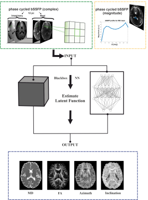
Figure 1. Scheme
of the neural network multi-parametric mapping pipeline. Real and imaginary
parts of the 12-point bSSFP phase-cycling data are fed voxelwise as input into
the NN (green box). For each voxel, a 3x3 window of nearest neighbors in the
axial plane is extracted leading to 216 input features. WM asymmetries in the
magnitude profile are shown for a representative ROI in corpus callosum (orange
box). The trained NNs enable voxelwise predictions of four diffusion metrics:
MD, FA, azimuth (Φ) and inclination (ϴ) (blue box).
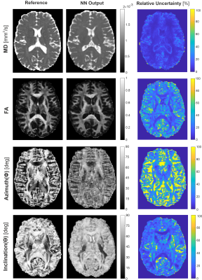
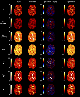
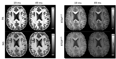
Figure 3. NN predictions (middle) are depicted
for a representative axial slice of a testing subject not included into NN
training in comparison to reference data (left) obtained with standard
SE-EPI-based DTI fitting. On the right, the corresponding relative uncertainty
maps of the NN are shown.
-
Rotation-Equivariant Deep Learning for Diffusion MRI
Philip Müller1, Vladimir Golkov1, Valentina Tomassini2, and Daniel Cremers1
1Computer Vision Group, Technical University of Munich, Munich, Germany, 2D’Annunzio University, Chieti–Pescara, Italy
We propose neural networks equivariant under rotations and translations for diffusion MRI (dMRI) data and therefore generalize prior work to the 6D space of dMRI scans. Our model outperforms non-rotation-equivariant models by a notable margin and requires fewer training samples.
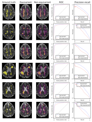
Segmentation of multiple-sclerosis lesions in six scans from the validation set. (a) Ground truth
of one example slice per scan, (b) predictions for that slice using our equivariant model, (c) predictions for that slice using the non-rotation-equivariant reference model with 3D convolutional layers, (e)
ROC curves of all models on the full scans, (f) precision-recall curves of all models on the full scans. While our equivariant model is very certain (yellow areas) at most positions, the non-rotation-equivariant model
has large areas of high uncertainty (purple areas).
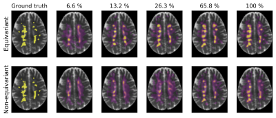
Segmentation of multiple-sclerosis lesions in a scan from the validation set (not used for training) using our equivariant (top) and the non-rotation-equivariant (bottom) model, both trained on reduced subsets of the training set (from left to right) with the ground truth segmentation in the left column. While our equivariant model achieves quite accurate segmentations when trained on 26.3% of the training scans, the segmentations of the non-rotation-equivariant model only start getting accurate when trained on 65.8% of the set, indicating better generalization of our model.
-
Improved image quality with Deep learning based denoising of diffusion MRI data
Radhika Madhavan1, Jaemin Shin2, Nastaren Abad1, Luca Marinelli1, J Kevin DeMarco3, Robert Y Shih3, Vincent B Ho3, Suchandrima Banerjee4, and Thomas K Foo1
1GE Global Research, Niskayuna, NY, United States, 2GE Healthcare, New York, NY, United States, 3Walter Reed National Military Medical Center and Uniformed Services University of the Health Sciences, Bethesda, MD, United States, 4GE Healthcare, Menlo Park, CA, United States
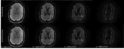
Diffusion MRI often suffers from low signal-to-noise ratio, especially for high b-values. This work proposes a deep learning based denoising method to address this limitation, allowing the use of high b-values as well as higher spatial resolution.
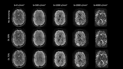
Figure 1: Diffusion weighted images for an example healthy volunteer showing improved SNR (separability of gray and white matter compartments in b-values >=2000 s/mm2) without spatial smoothing across multiple intensities of DL-based denoising.
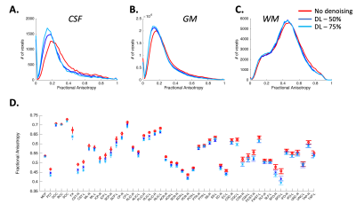
Figure 3: DL-based denoising improved differentiation across signal compartments while preserving quantitative tensor-based metrics. (A-C) Histogram analysis demonstrating distribution of FA values in whole brain CSF, Gray matter (GM) and WM. Quantitative diffusion metrics were compared across two level of DL denoising (50% and 75%). Results were consistent across both volunteers and across acquisitions. (D) FA values across 50 WM regions remain unchanged demonstrating that DL-based denoising maintains tensor-based quantitative metrics.
-
Deep learning based denoising for high b-value high resolution diffusion imaging
Seema S Bhat1, Pavan Poojar2, Hanumantharaju M C3, and Sairam Geethanath1,2
1Medical Imaging Research center, Dayananda sagar college of engineering, Bangalore, India, 2Columbia University in the City of New York, Newyork, NY, United States, 3Department of Electronic and Communications, BMS Institute of Technology and Management, Bangalore, India
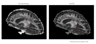
Deep learning based denoising of high b-value DWI was done in this work and we achieved PSNR (>32dB) for noise simulated DWI and image entropy(>7.17) for prospective DWI. Denoising can reduce acquisition time and increase resolution with smaller slice thickness.
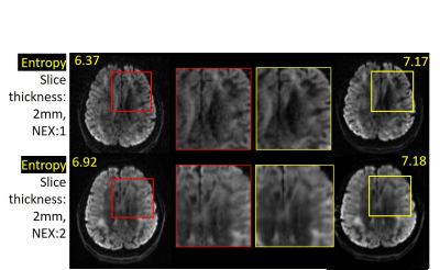
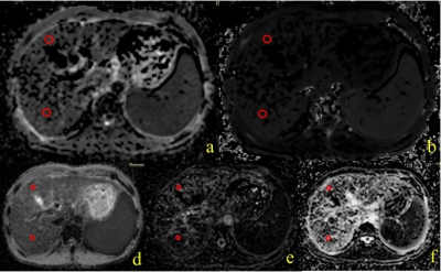
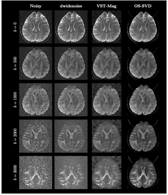
Figure 5: First column shows high b-value prospective DWI with slice thickness 2 mm, NEX=1, 2. More noise in test images can be observed with reduction in slice thickness. Last column shows their denoised counterparts. Noisy & denoised parts are magnified (highlighted with red and yellow squares) in second & third columns. Significant noise reduction and increase in entropy measures can be noted.
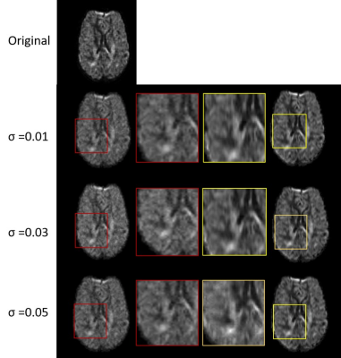
Figure 2: Visualization of Openneuro high b-value DWI denoising: First column (second row onwards) shows input images with Rician noise at σ =0.01,0.03 and 0.05 respectively. Last column shows denoised images. Noisy & denoised parts are magnified (highlighted with red and yellow squares respectively) in second & third columns. Significant reduction in noise can be observed in the denoised version.
-
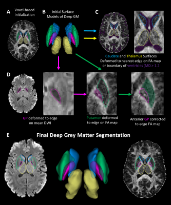
Microstructural White Matter Segmentation in Mild Traumatic Brain Injury Patients using DTI and a Deep 2D-UNet Ensemble
Brian McCrindle1,2, Nicholas Simard1,2, Ethan Samson2,3, Ethan Danielli 2,3, Thomas E. Doyle1,3,4, and Michael D. Noseworthy1,2,3
1Electrical and Computer Engineering, McMaster University, Hamilton, ON, Canada, 2Imaging Research Center, St. Joseph's Healthcare, Hamilton, ON, Canada, 3School of Biomedical Engineering, McMaster University, Hamilton, ON, Canada, 4Vector Institute, Toronto, ON, Canada
We develop a deep ensemble-based 2D-UNet framework for brain microstructural white matter damage segmentation. We show that ensembles perform the most reliably in out-of-distribution conditions even with minimal training data.
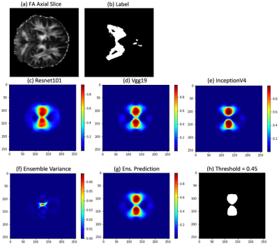
Example of an unseen slice fed into the ensemble model. (a) Normalized Axial FA Slice. (b) Z-Scoring label. (c – e) Model predictions for 2D-UNets with Resnet101, Vgg19, InceptionV4 Encoders with Dice scores 0.69, 0.69, 0.70 respectively. (f) Ensemble Predictive Uncertainty. (g) Ensemble Prediction. (h) Ensemble Prediction with “Optimal” Threshold and a Dice Score of 0.71.
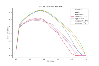
Dice-Score vs Threshold for all models with and without TTA. The ensemble performs most reliably over the threshold range.
-
Deep learning-based DWI Denoising method that suppressed the "instability" problem
Hayato Nozaki1,2, Yasuhiko Tachibana3, Yujiro Otsuka4, Wataru Uchida1,2, Yuya Saito1, Koji Kamagata1, and Shigeki Aoki1
1Department of Radiology, Graduate School of Medicine, Juntendo University, Tokyo, Japan, 2Graduate School of Human Health Sciences, Tokyo Metropolitan University, Tokyo, Japan, 3Department of Molecular Imaging and Theranostics National Institute of Radiological Sciences National Institutes for Quantum and Radiological Science and Technology, Chiba, Japan, 4Miliman, Tokyo, Japan
The deep learning-based method which can
effectively denoise DWI images almost without risked to output outliers due to
the instability problem in deep learning was developed and evaluated.
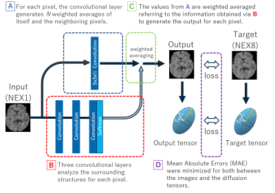
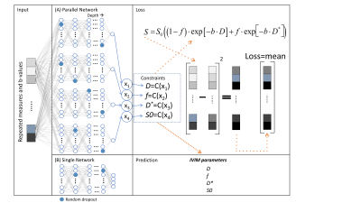
Figure 1. Outline of the neural network architecture.
The output value has small risk to become an
outlier because it is generated by the combination of the weighted averages for
the neighboring pixels in the original image. The loss to be minimized consists
of both the mean absolute error between the output and the target images and
the Euclid distance between the derived diffusion tensors for efficient
optimization.
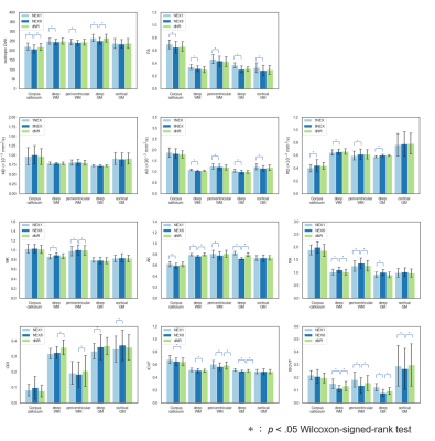
Figure 4. The results of the ROI-based
analysis.
dNR was closer to NEX8 than NEX1 in most
regions and parameter maps, and some significant differences between NEX1 and
NEX8 were resolved in between dNR and NEX8. However, dNR was far from NEX8 than
NEX1 in some combinations of the region and the parameter. Especially, in the
regions of deep white matter and periventricular white matter in ODI, the
difference compared to NEX8 was significant in dNR and not in NEX1.
-
Accelerating Brain Diffusion Tensor Imaging using Neural Networks: A Comparison of three Neural Networks
Yuhao Yan1,2 and Zheng Chang1,2
1Medical Physics Graduate Program, Duke University, Durham, NC, United States, 2Department of Radiation Oncology, Duke University, Durham, NC, United States
Neural networks can
accelerate brain DTI. Cascade-net out-performed U-net and PD-net, obtaining comparable
image quality as compared with the reference reconstructed from the full
k-space data on reconstruction of DTI images, ADC maps and FA maps.
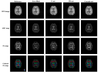
Figure 3. Illustration of DTI images, ADC maps, FA maps and colored FA maps of a
selected slice, from top to bottom row. Each column from left to right are
reference images reconstructed from full k-space data, images reconstructed
from zero-filled under-sampled k-space data, images reconstructed from
under-sampled k-space data using U-net, PD-net and Cascade-net.
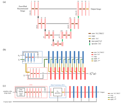
Figure 1.a. Structure of U-net.1,4 The number of filters in each layer is a quarter of the original
structure. Zero-padding is adapted to maintain the size of images in
convolutions. 1.b. Structure of PD-net.5 In this work,
the activation function PReLU non-linearity in the original structure was
substituted by ReLU non-linearity for consistency with U-net and Cascade-net.1
1.c. Structure of Cascade-net.2 The number of
filters was set as 48 in this work, which was 64 in the original structure.1
-
Accelerating Diffusion Tensor Imaging of the Rat Brain using Deep Learning
Ali Bilgin1,2,3,4, Loi Do1, Phillip A Martin2, Ethan Lockhart4, Adam S Bernstein1, Chidi Ugonna1, Laurel Dieckhaus1, Courtney Comrie1, Elizabeth B Hutchinson1, Nan-Kuei Chen1, Gene E Alexander5,6, Carol A Barnes5,7,8, and Theodore P Trouard1,3,5
1Biomedical Engineering, University of Arizona, Tucson, AZ, United States, 2Electrical and Computer Engineering, University of Arizona, Tucson, AZ, United States, 3Medical Imaging, University of Arizona, Tucson, AZ, United States, 4Program in Applied Mathematics, University of Arizona, Tucson, AZ, United States, 5Evelyn F. McKnight Brain Institute, University of Arizona, Tucson, AZ, United States, 6Departments of Psychology and Psychiatry, University of Arizona, Tucson, AZ, United States, 7Division of Neural System, Memory & Aging, University of Arizona, Tucson, AZ, United States, 8Departments of Psychology, Neurology and Neuroscience, University of Arizona, Tucson, AZ, United States
Deep
learning enables calculation of diffusion tensor metrics with up to ten-fold
reduction in scan time when imaging the rat brain.
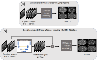
Figure1: (a) In
conventional DTI, acquired DWIs are first used to estimate the diffusion
tensor. The resulting tensor is used to compute the DTI metrics. (b) In
proposed DL-DTI, the acquired DWIs are first used to predict DWIs that were not
acquired. The acquired and predicted DWIs are used together for estimating the
diffusion tensor. The diffusion tensor is then used to compute the DTI metrics.
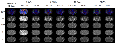
Figure 3: Comparison of DTI
metrics. Directionally Encoded Color (DEC), Fractional Anisotropy (FA), Mean Diffusivity
(MD), Axial Diffusivity
(AD), and Radial Diffusivity (RD) maps are shown for
a reference (N=64) dataset together with the same metrics obtained using the
conventional DTI (Figure 1(a)) and DL-DTI (Figure 1(b)) approaches using a varying
number of input DWIs. The metrics obtained from DL-DTI correspond well to those
obtained using the reference dataset even at high acceleration rates.
-
Automatic Detection of Nyquist Ghosts in Whole-Body Diffusion Weighted MRI Using Deep Learning
Alistair Lamb1, Anna Barnes2, Stuart A Taylor2, and Hui Zhang3
1Department of Medical Phyics and Biomedical Engineering, University College London, London, United Kingdom, 2Centre for Medical Imaging, University College London, London, United Kingdom, 3Centre for Medical Image Computing, University College London, London, United Kingdom
A supervised deep-learning
approach to detect the presence of Nyquist ghosts in axial DWI slices of the abdomen
is proposed with intent for use in improving the reproducibility of
quantitative ADC measurements in the body. A test accuracy of 81.5% was achieved.
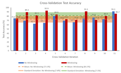
Figure 5: The percentage accuracy of the classifier on test
data for each of the 11 cross-validation iterations is shown, for both the
network trained on DWI slices with intensity values windowed between 0-25, and
for the network trained without windowing. The mean accuracy and corresponding
standard deviation across all 11 iterations is also shown for both cases.
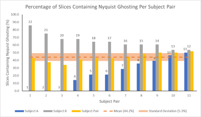
Figure 5: The
percentage of slices containing Nyquist ghosts is shown for each
pair of subjects. For each subject pair, the percentage for the constituent subjects are also shown, labelled
with the subject number. The mean (44.2%) across all subject pairs is given, along with the standard deviation (5.3%) which is much lower than that of slices containing Nyquist Ghosting in individual
subjects, as shown in Figure 2.
-
SRDTI: Deep learning-based super-resolution for diffusion tensor MRI
Qiyuan Tian1,2, Ziyu Li3, Qiuyun Fan1,2, Chanon Ngamsombat1, Yuxin Hu4, Congyu Liao1,2, Fuyixue Wang1,2, Kawin Setsompop1,2, Jonathan R Polimeni1,2, Berkin Bilgic1,2, and Susie Y Huang1,2
1Athinoula A. Martinos Center for Biomedical Imaging, Massachusetts General Hospital, Boston, MA, United States, 2Harvard Medical School, Boston, MA, United States, 3Department of Biomedical Engineering, Tsinghua University, Beijing, China, 4Department of Electrical Engineering, Stanford University, Stanford, CA, United States
- 1. Proposed
a deep learning-based super-resolution method for DTI.
- 2. Employed a very deep convolutional
neural network, residual learning, and multi-contrast imaging.
- 3. High-quality results similar to
high-resolution ground truth and superior to those from image interpolation.
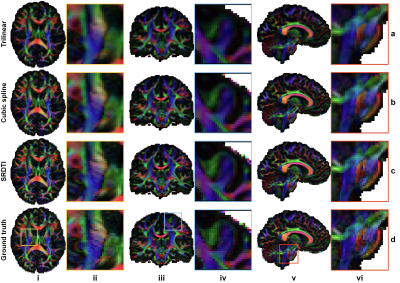
Figure 3. Direction-encoded
fractional anisotropy maps. Fractional anisotropy maps color
encoded by the primary eigenvector (red: left–right; green: anterior–posterior;
blue: superior–inferior) derived from the diffusion tensors fitted using interpolated
data (a, b), SRDTI super-resolution data (c), and ground-truth high-resolution
data (d) along axial, coronal and sagittal directions, showing
regions-of-interest in the internal capsule (i, ii), cerebral cortex (iii, iv)
and pons (v, vi), respectively.
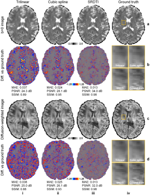
Figure 2. Image results. b=0 images (row a) and diffusion-weighted images (DWIs) (row
c) along one direction of the six optimized diffusion-encoding directions (i.e.,
[0.91, 0.416, 0]) from interpolated data (i, ii) (interpolated data using cubic
spline is the input to SRDTI), SRDTI output data (iii), ground-truth
high-resolution data (iv), and their residuals comparing to the ground-truth high-resolution
images (rows b, d). A region-of-interest in the deep white matter (yellow
boxes) is displayed in enlarged views (rows, b, d, column iv).
-
Inferring Diffusion Tensors on Unregistered Cardiac DWI Using a Residual CNN and Implicitly Modelled Data Prior
Jonathan Weine1, Robbert J. H. van Gorkum1, Christian T. Stoeck1, Valery Vishnevskiy1, Thomas Joyce1, and Sebastian Kozerke1
1Institute for Biomedical Engineering, University and ETH Zurich, Zürich, Switzerland
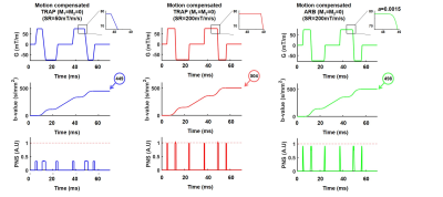
We present a feasibility study of training a residual
CNN on simulated data to infer diffusion tensors from unregistered free breathing
single-shot 2nd order
motion-compensated diffusion-weighted SE-EPI data. Improvement in resulting
parameter maps at myocardial borders is demonstrated.
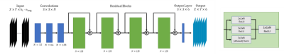
Figure 1: Architecture design of
the proposed residual CNN. Input is 144 stacked diffusion-weighted
magnitude images, normalized to the mean LV intensity of the first image. The final output
6 channels represents the tensor entries. Convolutional layers (blue) have a
$$$3\times3\times N$$$
kernel and ReLU activation. The residual blocks (green)
consist of the parallel paths with
different kernel sizes. The outputs are concatenated and reduced 1
convolution layer to match the input channels.
The output of a residual block is added to the skip
connection and fed to the next block.
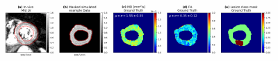
Figure 2: Illustration of the
simulated training data and visual comparison to real in vivo data. (a)
Animation of single averages for each linear diffusion-weighting and (b)
example of the correspondingly simulated and LV-masked training dataset. The
red contours show a dilated LV-mask in which the inference on the unregistered
data is performed. (c-d) Maps of mean MD, FA as well as an artificial lesion map resulting serving as ground truth of
the simulated dataset.
-
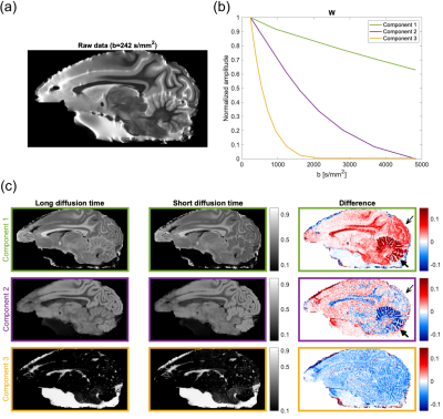
Learning the relationship between human brain tissue microstructure and diffusion MRI data
Emmanuelle Weber1, Christoph Leuze1, Daniel A. N. Barbosa1, Gustavo Chau Loo Kung1, Kalanit Grill-Spector1, and Jennifer A. McNab1
1Stanford, Stanford, CA, United States
Feasibility
study of a machine learning direct prediction of tissue microstructure from raw
diffusion MRI data. We attempted to predict the well-understood main fiber
orientation from both simulated and dMRI-3D histology dataset.
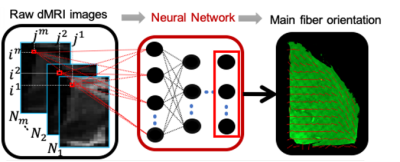
Figure 1: Deep learning
framework aiming at predicting the microstructural features from raw diffusion
MRI (dMRI) data using histology images as ground truth. Example of prediction
of main fiber orientation from previously acquired data on human thalamus.
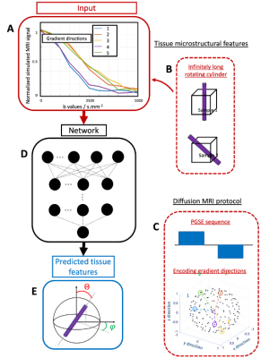
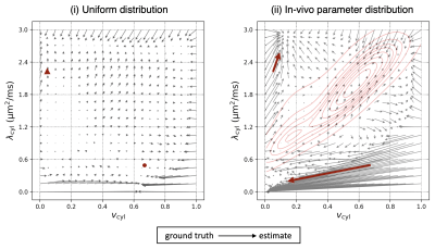
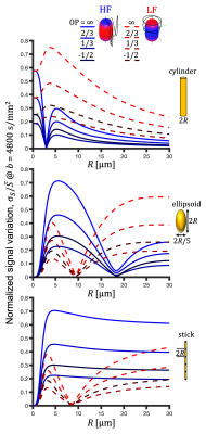
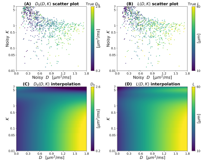
Figure
2: Summary of the whole pipeline that enables to
predict a single simulated fiber orientation using deep learning. A) Normalized
dMRI signal from an B) infinitely long rotating cylinder as a function of the
C) PGSE sequence b values for different gradient orientation. D) This signal is
then fed to a neural network to predict the E) orientation of the cylinder
given by the spherical angles theta and phi.
-
Patch-CNN-DTI: Data-efficient high-fidelity tensor recovery from 6 direction diffusion weighted imaging.
Tobias Goodwin-Allcock1, Ting Gong1, Robert Gray2, Parashkev Nachev2, and Hui Zhang1
1Centre for Medical Image Computing (CMIC), UCL, London, United Kingdom, 2High-Dimensional Neurology, University College London Queen Square Institute of Neurology, London, United Kingdom
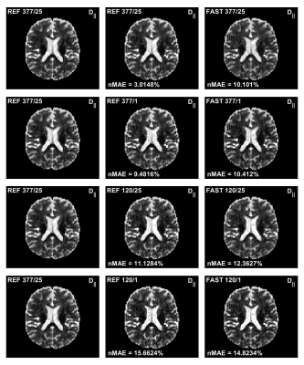
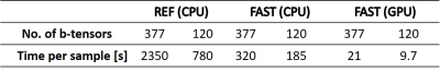
Proposed Patch-CNN-DTI as a method for estimating accurate
diffusion tensors from as few as 6 diffusion-weighted images (DWI) with only
one training subject, which outperforms conventional fitting with twice the
number of DWIs.
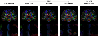
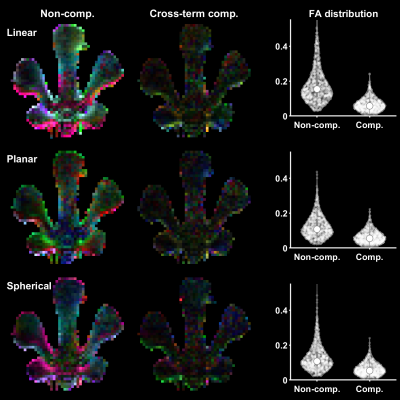
Figure 2) Top are the FA
weighted colour maps of the primary direction of diffusion. The motor tract,
highlighted in yellow, is enlarged at the bottom where the primary directions
of diffusion are illustrated as colour encoded sticks. The sticks are masked such
that only WM voxels remain, determined by FA>0.2. Estimations from
Patch-CNN are visually more similar to the GT for both RGB colourmap and sticks.
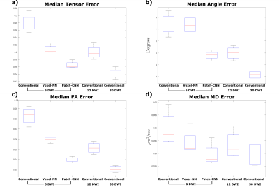
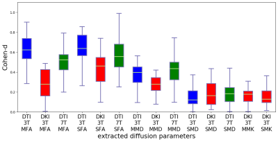
Figure 4) Boxplots
computed over the medians of errors for each of the 4 testing subjects. For
(a,c,d) the median error is computed across all of the brain voxels at each
subject. For (b) median error is computed for each subject across voxels for
which the primary direction of diffusion is well defined, where the linearity
coefficient9>0.6.
-
Rapid Multi-slice STEAM Diffusion Imaging with a Prepared Gradient Echo Echoplanar Sequence
David C Alsop1,2, Manuel Taso1,2, and Arnaud Guidon3
1Radiology, Beth Israel Deaconess Medical Center, Boston, MA, United States, 2Radiology, Harvard Medical School, Boston, MA, United States, 3Global MR applications and workflow, GE Healthcare, Boston, MA, United States
We propose a non-selective preparation of a
conventional gradient echo echoplanar sequence that enables the rapid
acquisition of many slices. Initial application to the brain readily enabled up
to 32 slice acquisition within a single TR.
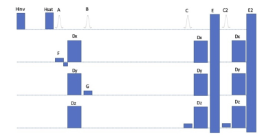
Figure 1. Schematic diagram of the nonselective STEAM
prepared multislice echoplanar sequence.
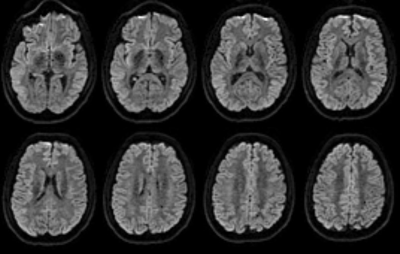
Figure 2: Example multi-slice b=1000 diffusion weighted
images after correction for differential slice delays by geometric averaging.
-
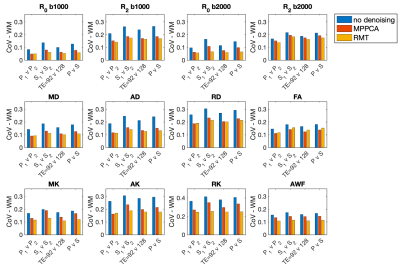
Multi-band in Diffusion MRI: Can we go too fast?
Arun Venkataraman1, Benjamin Risk2, Deqian Qiu3,4, Jianhui Zhong1,5, and Zhengwu Zhang6
1Physics and Astronomy, University of Rochester, Rochester, NY, United States, 2Biostatistics and Bioinformatics, Emory University, Atlanta, GA, United States, 3Radiology and Imaging Sciences, Emory University School of Medicine, Atlanta, GA, United States, 4Biomedical Engineering, Emory University, Atlanta, GA, United States, 5Imaging Sciences, University of Rochester Medical Center, Rochester, NY, United States, 6Biostatistics and Computational Biology, University of Rochester Medical Center, Rochester, NY, United States
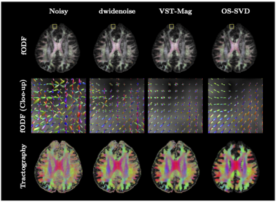
In this study, we found that slice and phase acceleration lead to increased noise amplification. This leads to worse DTI fitting and instability of tractography that is preferentially seen in the frontal areas, with relative sparing of the occipital areas.
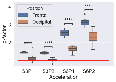
Figure 2 g-factor calculated for all accelerated acquisitions, red line indicates g-factor of 1, which represents the SNR of the unaccelerated (S1P1) dMRI acquisiton. p-values indicated by asterisks and were calculated using a paired t-test, in this figure, all p < 0.0001 (****).
-
A unified framework for estimating diffusion kurtosis tensors with multiple prior information
Li Guo1,2,3, Lyu Jian2,3, Yingjie Mei4, Mingyong Gao1, Yanqiu Feng2,3, and Xinyuan Zhang2,3,5
1Department of MRI, The First People’s Hospital of Foshan (Affiliated Foshan Hospital of Sun Yat-sen University), Foshan, China, 2School of Biomedical Engineering, Southern Medical University, Guangzhou, China, 3Guangdong Provincial Key Laboratory of Medical Image Processing, Southern Medical University, Guangzhou, China, 4Philips Healthcare, Guangzhou, China, 5Guangdong-Hong Kong-Macao Greater Bay Area Center for Brain Science and Brain-Inspired Intelligence, Guangzhou, China
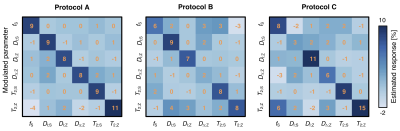
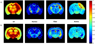
The unified framework
that integrates multiple prior information including nonlocal structural
self-similarity, local spatial smoothness, physical relevance of DKI model, and
noise characteristic of magnitude diffusion images can improve the accuracy of
DKI tensor estimation.
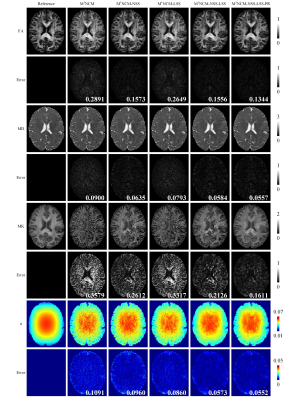
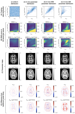
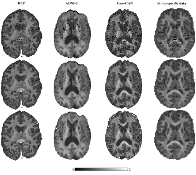
Figure 3. FA, MD, MK, noise SD (σ) maps and
their corresponding error maps of the M1NCM-based methods, using the
simulated data with unstationary noise level of 0.02. The error maps show the
absolute difference between the reference parameters and the estimated
parameters. The RMSE of each parameter map is shown in the right bottom of its
error map. The unit of the MD is ×10-3 mm2/s.
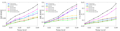
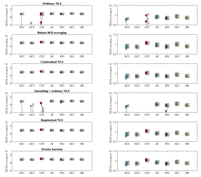
Figure 1. RMSE comparisons of FA,
MD, MK maps estimated with the UVNLM-NLS, UVNLM-CWLLS, M1NCM, M1NCM-NSS,
M1NCM-LSS, M1NCM-NSS-LSS, and M1NCM-NSS-LSS-PR
algorithms, using the simulated datasets with stationary and fixed noise levels
of 0.02-0.09.
-
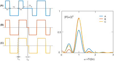
Influence of electrocardiogram signal triggering on filter exchange imaging
Julian Rauch1,2, Dominik Ludwig1,2, Frederik B. Laun3, and Tristan A. Kuder1
1Division of Medical Physics in Radiology, German Cancer Research Center (DKFZ), Heidelberg, Germany, 2Faculty of Physics and Astronomy, Heidelberg University, Heidelberg, Germany, 3Institute of Radiology, University Hospital Erlangen, Friedrich-Alexander-Universität Erlangen-Nürnberg (FAU), Erlangen, Germany
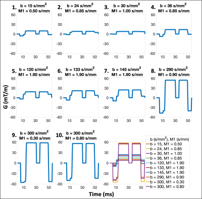
The
signal stability of AXR measurements is slightly improved when suppressing
pulsation-induced variations by ECG triggering. However, pulsation does not
seem to be the main source of signal variations.
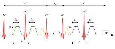
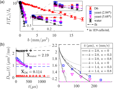
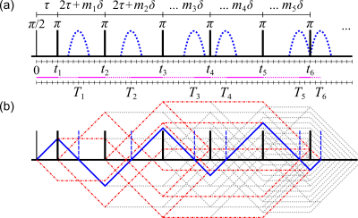
Figure
1: Schematic
representation of a filter exchange imaging (FEXI) sequence using two pulsed
gradient spin echo (PGSE) blocks. The first gradient pair used as the FEXI
filter is followed by a varying mixing time during which
the magnetization is longitudinally stored while transversal components are
dephased. Before and after the second and third radiofrequency pulse,
respectively, gradients to choose the right echo path are applied. The second
gradient pair is a standard diffusion weighting. This block is followed by an
echo planar imaging (EPI) readout.
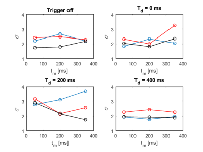
Figure
2: Comparison of the standard deviations σ resulting from the different trigger
experiments. No diffusion weighting was applied (b = 0 s/mm2).
The three used
orthogonal diffusion encoding directions (2/3, 2/3, 1/3), (1/3, 2/3, 2/3) and (2/3, 1/3, 2/3)
are depicted in blue,
red and black, respectively.
-
Improved parameter estimation for non-Gaussian IVIM using an unbiased vector non-local means
Lyu Jian1,2, Xinyuan Zhang1,2,3, Yingjie Mei4, and Li Guo1,2,5
1School of Biomedical Engineering, Southern Medical University, Guangzhou, China, 2Guangdong Provincial Key Laboratory of Medical Image Processing, Southern Medical University, Guangzhou, China, 3Guangdong-Hong Kong-Macao Greater Bay Area Center for Brain Science and Brain-Inspired Intelligence, Guangzhou, China, 4Philips Healthcare, Guangzhou, China, 5Department of MRI, The First People’s Hospital of Foshan (Affiliated Foshan Hospital of Sun Yat-sen University), Foshan, China
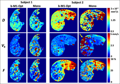
To improve the accuracy and precision of parameter
estimation for NG-IVIM, we propose to use an unbiased vector non-local means
(UVNLM) filter to denoise and correct the noise bias before NG-IVIM model
fitting.
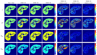
Fig.
4. f, D*, Dapp, Kapp maps and their corresponding
error maps of the proposed UVNLM-NLS method. The error maps show the absolute
difference between the reference parameters and the estimated parameters.
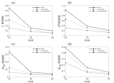
Fig. 1. RMSE comparisons
of f, D*, Dapp, Kapp
maps estimated with the conventional NLS, the PCA-NLS, the proposed UVNLM-NLS
method.
-
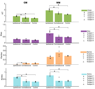
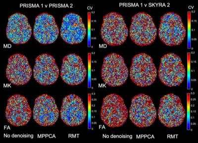
Evaluation of quantitative MRI parameters reproducibility across a major scanner upgrade: spinal cord diffusion weighted (DW) imaging
Ratthaporn Boonsuth1, Marco Battiston1, Francesco Grussu1,2, Marios Yiannakas1, Torben Schneider3, Rebecca Samson1, Ferran Prados1,4,5, and Claudia A. M. Gandini Wheeler-Kingshott1,6,7
1NMR research Unit, Queen Square MS Centre, Department of Neuroinflammation, UCL Queen Square Institute of Neurology, London, United Kingdom, 2Radiomics Group, Vall d’Hebron Institute of Oncology, Vall d’Hebron Barcelona Hospital Campus, Barcelona, Spain, 3Philips Healthcare, Guildford, Surrey, United Kingdom, 4Centre for Medical Image Computing, Medical Physics and Biomedical Engineering, University College London, London, United Kingdom, 5E-Heath Centre, Universitat Oberta de Catalunya, Barcelona, Spain, 6Department of Brain & Behavioural Sciences, University of Pavia, Pavia, Italy, 7Department of Brain Connectivity Centre Research Department, IRCCS Mondino Foundation, Pavia, Italy
The
diffusion-derived metrics are reproducible, with no significant differences
between pre- and post-upgrade in spinal cord, white matter, and grey matter.
Following a major scanner upgrade at a single site, diffusion measurements were
found not to differ substantially
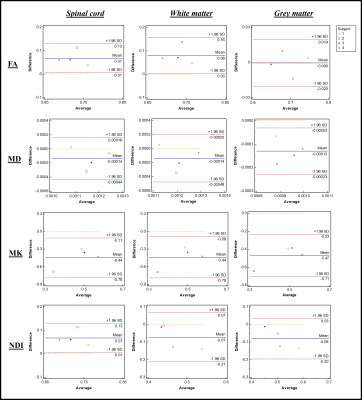
Figure 1.
Bland–Altman plots of four diffusion metrics for 3 different ROIs, namely whole
spinal cord area, white matter, and grey matter. The x and y-axes represent,
respectively, average, and mean differences between pre- and post-upgrade. The
blue lines show the mean of the differences, while the pairs of dotted red
lines denote the 95% confidence intervals.
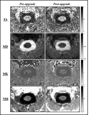
Figure 2. Parametric maps for fractional anisotropy (FA),
mean diffusity (MD), mean kurtosis (MK) and neurite density index (NDI) from
a single subject obtained pre- and post-upgrade.
-
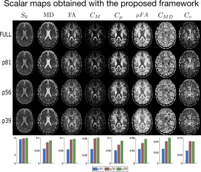
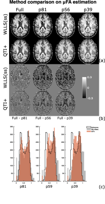
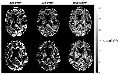
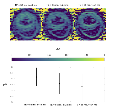
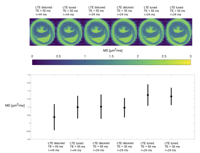
High-resolution microstructural imaging in the human hippocampus with b-tensor encoding and zoomed imaging
Jiyoon Yoo1, Leevi Kerkelä1, Patrick W. Hales1, Kiran K. Seunarine1, Iulius Dragonu2, Enrico Kaden1, and Christopher A. Clark1
1UCL Great Ormond Street Institute of Child Health, London, United Kingdom, 2Siemens Healthcare Ltd, Frimley, United Kingdom
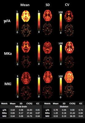
All-in-one sequence for microstructural imaging in the hippocampus, providing high-resolution images for localisation of hippocampal subregions and fitting of standard and advanced diffusion models.
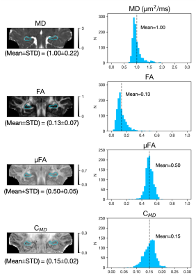
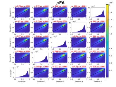
Figure 3. Derived microstructural maps and parameters. From top to bottom: Mean diffusivity (MD) from diffusion kurtosis fit, fractional anisotropy (FA) calculated from diffusion kurtosis fit, microscopic fractional anisotropy (μFA) from QTI, normalised size variance (CMD) from QTI. STD=standard deviation.
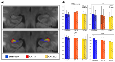
Figure 4. (A) Mean diffusion-weighted LTE image at b-value of 1000 s/mm2 shows contrast within the hippocampal subregions. Subregions were manually segmented for subiculum (blue), Cornu Ammonis (CA) regions CA1-3 (red) and CA4 with dentate gyrus (DG, yellow). (B) Microstructural parameters were calculated in each subregion; Subiculum, CA1-3 and CA4/DG.