-
Pipeline for processing EEG data acquired during block-design simultaneous EEG-fMRI-ASL study
Balu Krishnan1, Wanyong Shin2, Ajay Nemani2, Anna Crawford2, and Mark Lowe2
1Epilepsy Center, Cleveland Clinic Foundation, CLEVELAND, OH, United States, 2Mellen Center, Cleveland Clinic Foundation, CLEVELAND, OH, United States
EEG data acquired during EEG-fMRI studies are prone to
multiple artifacts. We detail an EEG artifact reduction
pipeline in a block design task paradigm during a BOLD/ASL sequence. Data
processed using the pipeline shows high fidelity and is comparable to data acquired outside the scanner.
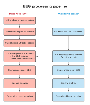
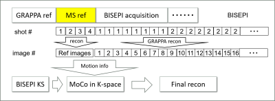
Figure 1: Processing pipeline for EEG
acquired inside and outside MRI scanner for simultaneous EEG-fMRI-ASL
experiment
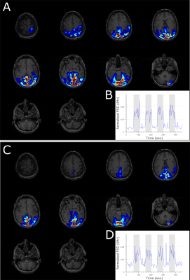
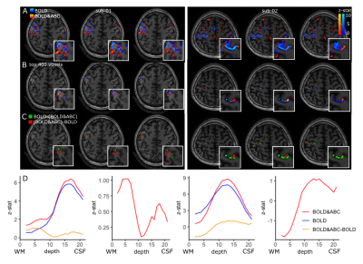
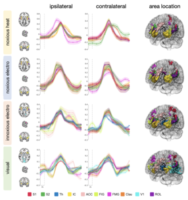
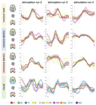
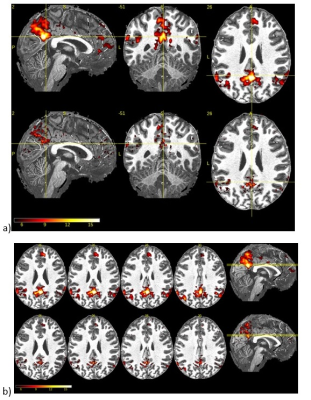
Figure 4: Generalized linear modeling of
the normalized power spectrum estimated from EEG while the subject is
performing a visual task showed activation in the visual cortex for EEG
recorded both (A) outside and (C) inside the scanner. The corresponding mean dynamic
spectral density function for the activated sources is shown in B and D. Grey area denotes time segments where the subject is
performing the visual task.
-
Are BOLD signal amplitude and synchronous low frequency fluctuations of EEG power related?
Wanyong Shin1, Balu Krishnan2, Ajay Nemani1, Anna Crawford1, and Mark J Lowe1
1Radiology, Cleveland Clinic, Cleveland, OH, United States, 2Epilepsy, Cleveland Clinic, Cleveland, OH, United States
In this study, we compare low-frequency fluctuation of theta to beta ratio (TBR) in the resting-state motor network with calibrated fMRI. The temporal fluctuation of TBR could be a potential index to investigate the resting-state brain networks in simultaneous EEG-fMRI studies.
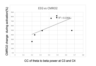
Fig 4. X and Y axes represent Pearson correlation coefficient of theta to beta fluctuation between C3 and C4 in the resting state, and estimated CMRO2 values in activated left M1 ROI.
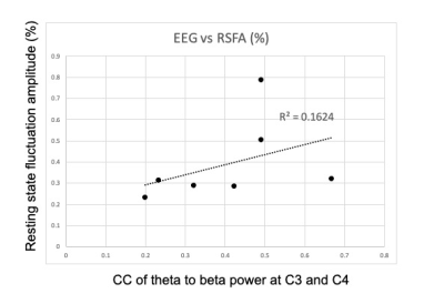
Fig 5. X and Y axes represent Pearson correlation coefficient of theta to beta fluctuation between C3 and C4 in the resting state, and percentage resting state fluctuation amplitude (RSFA) in activated left M1 ROI.
-
Deriving an EEG model to predict the activity of the default mode network measured by fMRI
Marta Xavier1, Inês Esteves1, Athanasios Vourvopoulos1, Ana R Fouto1, Amparo Ruiz-Tagle1, Raquel Gil-Gouveia2, and Patrícia Figueiredo1
1Department of Bioengineering, Institute for Systems and Robotics, Lisbon, Portugal, 2Neurology Department, Hospital da Luz, Lisbon, Portugal
We demonstrated the viability of the proposed EEG models in predicting the simultaneous fMRI signal from the DMN. We showed that measures of similarity between the predicted and target BOLD signal significantly varied with the model used.
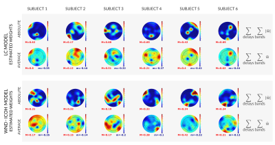
Figure 3: Topographic representation of the estimated model weights, obtained independently for each subject (columns), for the models LC and WD-Icoh (rows). Bottom: estimated weights (w), summed across frequency bands and delays. Top: absolute values of the estimated weights (|w|), summed across frequency bands delays. Minimum and maximum values indicated for each map with m (blue) and M (red).
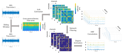
Figure 2: Extraction of the features for the WD-Icoh model. The cross-spectrum was estimated for a hundred frequency values (1-30Hz) in a sliding window of 4s (250ms step size). In each window, the expected value of the cross-spectral density was estimated using Welch's periodogram method. The imaginary part of coherency (Icoh) between each channel pair was estimated and filtered for significance. The weighted degree of each channel was then estimated and averaged for the δ, θ, α and β band.
-
Optimizing EEG source reconstruction with concurrent fMRI-derived spatial priors
Rodolfo Abreu1, Júlia F. Soares1, Sónia Batista2,3, Lívia Sousa2,3, Miguel Castelo-Branco1,3, and João Valente Duarte1,3
1Coimbra Institute for Biomedical Imaging and Translational Research (CIBIT), Institute for Nuclear Sciences Applied to Health (ICNAS), University of Coimbra, Coimbra, Portugal, 2Neurology Department, Centro Hospitalar e Universitário de Coimbra, Coimbra, Portugal, 3Faculty of Medicine, University of Coimbra, Coimbra, Portugal
Our comparison
revealed that combining a beamformer for EEG source reconstruction with
fMRI-derived spatial priors improves the quality of the reconstructions in
terms of the overlap with atlas-based anatomical brain regions known
to be involved in similar tasks, and RSN templates.
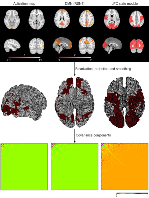
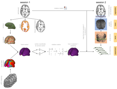
Fig. 2: Deriving covariance components (CCs) from fMRI spatial priors. The
3D fMRI spatial priors are first binarized, projected onto the 2D cortical
surface using nearest-neighbor interpolation and smoothed using the Green’s
function. The associated CCs are then obtained by computing the outer product.
For visualization purposes, the temporally reduced CCs are illustrated, by
applying the same temporal projector considered when reducing the EEG data
prior to its reconstruction.
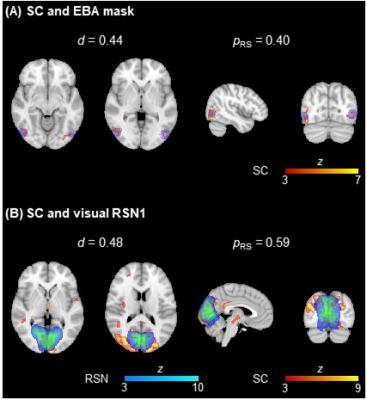
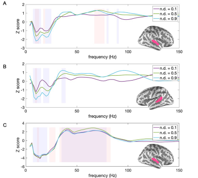
Fig. 3: Illustration of the overlap between two EEG SCs (in red-yellow) and (A)
the EBA mask (in blue) and (B) a visual RSN (in blue-light blue) from 15. The dice coefficient d and the proportion of the ROIs contained in the respective SCs
are also depicted.
-
Evaluation of ECG-derived respiration signals in simultaneous EEG-fMRI acquisitions
Inês Esteves1, Ana R. Fouto1, Amparo Ruiz-Tagle1, Athanasios Vourvopoulos1, Marta Xavier1, Nuno A. Silva2, Raquel Gil-Gouveia3, Agostinho Rosa1, and Patrícia Figueiredo1
1ISR-Lisboa and Department of Bioengineering, Instituto Superior Técnico – Universidade de Lisboa, Lisbon, Portugal, 2Learning Health, Hospital da Luz, Lisbon, Portugal, 3Neurology Department, Hospital da Luz, Lisbon, Portugal
The feasibility of deriving ECG-derived respiration (EDR) signals for EEG-fMRI was shown, by comparison with the true respiratory signal. KPCA and PCA methods achieved the best performance, though EDR-based fMRI regressors should be further studied.
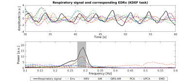
Figure 1: Respiratory signal and the corresponding EDRs obtained with different methods, from a representative subject performing the KDEF task: signal time courses over a period of 30s (top); and power spectra for the whole signal (bottom). The grey rectangle corresponds to the frequency band around the respiratory frequency for which the power is at least half of the maximum power.
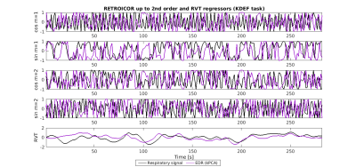
Figure 3: fMRI respiratory regressors, from a representative subject performing the KDEF task (same as in Fig.1): RETROICOR components obtained from the Fourier expansion up to the 2nd order of the respiratory phases (cosines and sines of order m=1,2); and respiratory volume per time (RVT), convolved with the respiratory response function [D], obtained from the measured respiratory signal (black) and the EDR signal estimated using the kPCA method (purple).
-
Closed-Loop tACS-fMRI: Online Optimization of tACS Stimulation to Enhance Fronto-parietal Connectivity
Beni Mulyana1,2, Aki Tsuchiyagaito1, Jared Smith1, Masaya Misaki1, Samuel Cheng2, Martin Paulus1, Hamed Ekhtiari1, and Jerzy Bodurka1
1Laureate Institute for Brain Research, Tulsa, OK, United States, 2Electrical and Computer Engineering, University of Oklahoma, Tulsa, OK, United States
Online optimization of tACS stimulation enhances
fronto-parietal connectivity, also selectively improves working memory in
healthy group as compared to control group. This study supports feasibility of
concurrent tACS-fMRI stimulation and measurement.
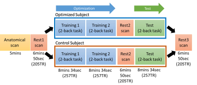
Overview of the closed-loop
tACS-fMRI-tACS runs. Training 1 and 2 on the experimental subject will find the
tACS parameters (frequency and phase) with the highest frontoparietal
connectivity. Otherwise, training 1 and 2 on the control subject will find the
tACS parameters (frequency and phase) with the lowest frontoparietal
connectivity.
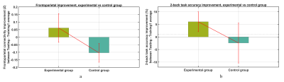
a. On testing – training1 average, The experimental group showed higher improvement of frontoparietal connectivity rather than control group [experimental group: mean=0.06, SD=0.09; control group: mean=-0.1, SD=0.06; t(9)=3.31, p=0.009]. b. On the same measurement (testing – training1 average), the experimental group showed higher improvement of 2-back task accuracy rather than control group [experimental group: mean=6.02, SD=3.96; control group: mean=-2.41, SD=7.95; t(9)=2.30, p=0.047].
-
Functional MRI of the excitatory and inhibitory neuromodulations by transcranial magnetic stimulation at the human sensorimotor cortex
Hsin-Ju Lee1,2, Mikko Nyrhinen3, Risto J. Ilmoniemi3, and Fa-Hsuan Lin1,2,3
1Physical Sciences Platform, Sunnybrook Research Institute, Toronto, ON, Canada, 2Department of Medical Biophysics, University of Toronto, Toronto, ON, Canada, 3Department of Neuroscience and Biomedical Engineering, Aalto University, Espoo, Finland
We measured fMRI signals caused by
excitatory and inhibitory TMS neuromodulations at the human primary motor
cortex. The primary motor cortex had fMRI signal after excitatory TMS. The
supplementary motor area had fMRI signals in both modulations.
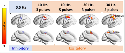
Figure 3. Distributions of significant fMRI signal changes in the individual TMS conditions. Positive fMRI signals were found at the SMC ipsilateral to the TMS target locus in all 10- and 30-Hz conditions, but not in the 0.5-Hz condition. The fMRI signal in the SMA was significantly increased in the 10-Hz–5-ppb, 30-Hz–3-ppb, and 30-Hz–5-ppb conditions.
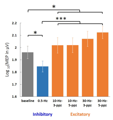
Figure 2. Log-transformed MEP amplitudes in the baseline
and in the individual TMS conditions. Significant MEPs were detected in all
conditions. The log-transformed MEP amplitude in the LF condition was
significantly smaller than in the baseline and HF conditions. In contrast, the
log-transformed MEP amplitude in the HF condition was significantly larger than
in the baseline. Error bars denote standard errors of the mean (SEM). *: p <
.05. ***: p < .001.
-
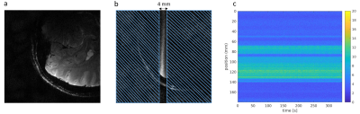
Intraoperative arterial spin labeling (iASL) reliably depicts functional networks during neurosurgery
Thomas Lindner1, Hajrullah Ahmeti2, Michael Helle3, Olav Jansen4, Michael Synowitz2, and Stephan Ulmer4,5
1University Hospital Hamburg-Eppendorf, Hamburg, Germany, 2Neurosurgery, University Hospital Schleswig-Holstein, Kiel, Germany, 3Tomographic Imaging Department, Philips Research Laboratories, Hamburg, Germany, 4Department of Radiology and Neuroradiology, University Hospital Schleswig-Holstein, Kiel, Germany, 5Radiology, Kantonsspital Winterthur, Winterthur, Switzerland
During neurosurgery, it is crucial to spare functional areas. Thsi can be achieved by using perfusion iamging to visualize the tumor area as well as using resting state fMRI to map active regions. The presented technique allows for both in a single sequence.
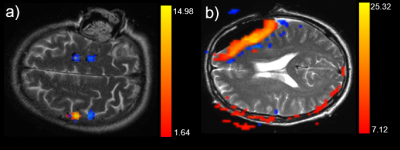
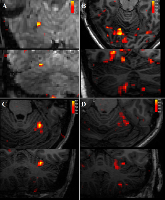
Figure 1: Representative examples of the activation of
the motor cortex (a) and false activation patterns in the resection cavity (b)
overlaid on T2 images.
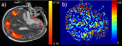
Figure 2: Example of the default mode network (a)
overlaid on a T2 image and the corresponding ASL perfusion (b). Note that in
the frontal area (medial prefrontal cortex and anterior cingulate cortex) no
default mode activation is visible as compared to the standard situation. The
inferior parietal cortex and cingulate cortex as well as the precuneus are visualized
as expected.
-
Visualizing Resting State Networks using Arterial Spin Labeling– Investigating the influence of Label and Control datasets
Thomas Lindner1, Michael Helle2, Olav Jansen3, and Stephan Ulmer3,4
1University Hospital Hamburg-Eppendorf, Hamburg, Germany, 2Tomographic Imaging Department, Philips Research Laboratories, Hamburg, Germany, 3Department of Radiology and Neuroradiology, University Hospital Schleswig-Holstein, Kiel, Germany, 4Radiology, Kantonsspital Winterthur, Winterthur, Switzerland
In this study, the effects of separating the label and control
condtion from an Arterial Spin Labeling dataset used for resting state
mapping was investigated and no differences between the label and the
control condition could be found.
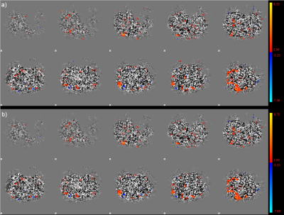
Figure 1: Example of one
dataset in which the control (a) and the label (b) images were post-processed
individually. There are only subtle differences visible and small deviations in
signal strength showing that there are no differences to be expected in
interpreting the data.
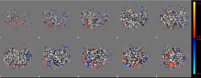
Figure 2: Same dataset as used
in figure 1, but this time both label and control images have been used for
processing, i.e. 80 datapoints (40 pairs) per slice were used. The patterns are
similar yet appear better delineated showing the higher statistical power of
this approach. Interestingly, the patter in the bottom middle image is not
visible in this result, suggesting that it is a false-positive activation in
the datasets with less datapoints.
-
Assessing intersubject BOLD synchronization and BOLD-CBF coupling using movie fMRI
Kaden T Shearer1, Allen A Champagne2, Nicole S Coverdale1, Ingrid S Johnsrude3, and Douglas J Cook4
1Centre for Neuroscience Studies, Queen's University, Kingston, ON, Canada, 2Department of Medicine, Queen's University, Kingston, ON, Canada, 3The Brain and Mind Institute, University of Western Ontario, London, ON, Canada, 4Department of Surgery, Queen's University, Kingston, ON, Canada
Compared to resting state, movie fMRI improves intersubject synchronization of the BOLD signal; however, no increases in BOLD-CBF coupling were observed. Improved ASL signal resolution and reduced noise may be required for differences in BOLD-CBF coupling to be revealed.
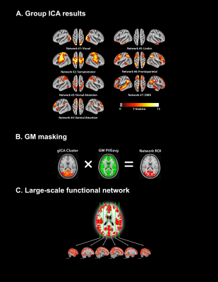
Figure 2. Schematic summarizing the workflow for establishing the large-scale functional ROI. (A) gICA was performed using FSL’s MELODIC11 with the number of pre-set spatial dimensions set to 50. Identified sub-networks were identified using the 7-network functional atlas13 and were thresholded at |t| > 4. (B) GM voxels were isolated by multiplying each identified sub-network by the subject’s GM partial volume estimation (PVE) mask, thresholded at 0.5. (C) The large-scale functional network mask was generated by spatially concatenating each identified GM sub-network.
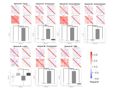
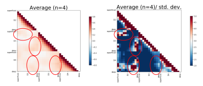
Figure 4. Summary of intersubject BOLD synchronization for the various networks analyzed. In each correlation matrix, the rows/columns correspond to the average BOLD timeseries for a given subject. The values at each row/column intersection correspond to the Pearson R correlation between the BOLD signal for subject x and subject y. Correlation matrices were compared statistically using a univariate ANOVA (* = P < .05; ** = P < .01; *** = P < .001).
-
Dynamic neurometabolic and functional changes in the dorsolateral prefrontal cortex in a working memory: a combined 1H fMRS and fMRI study
Hyerin Oh1,2, Ben Babourina-Brooks1,2,3, Adam Berrington2,3, Dorothee P Auer1,2,3, Henryk Faas1,2, and JeYoung Jung4
1Division of Clinical Neuroscience, School of Medicine, University of Nottingham, Nottingham, United Kingdom, 2Sir Peter Mansfield Imaging Centre, University of Nottingham, Nottingham, United Kingdom, 3NIHR Nottingham Biomedical Research Centre, Queen’s Medical Centre, University of Nottingham, Nottingham, United Kingdom, 4School of Psychology, University of Nottingham, Nottingham, United Kingdom
Working memory task increased Glx concentrations in the DLPFC. Dynamic changes of Glx were associated with increased regional activity in the DLPFC as well as task performance in working memory.
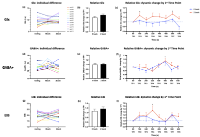
Figure 2. (a), (d), (g) individual difference of Glx, GABA+, EIB in each condition (resting, 0 back, 2 back). (b), (e), (h) averaged relative Glx, GABA+, EIB change by T1. (c), (f), (i) dynamic relative Glx, GABA+, EIB change by T1. * p < 0.05
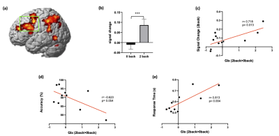
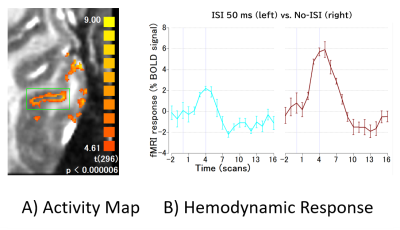
Figure 3. (a) fMRI results: 2-back > 0-back. A green box indicates the region of Interest (ROI) placement. (b) BOLD signal changes during 0 back and 2 back in the DLPFC ROI. (c) A positive correlation between signal change during 2-back and Glx changes (2-back > 0-back). (d) A negative correlation between 2-back task accuracy and Glx changes (2-back > 0-back). (e) A positive correlation between 2-back task response time and Glx changes (2-back > 0-back). *** p <0.001
-
WM motor learning can be detected using low frequency oscillations in time series functional MRI
Tory Frizzell1, Elisha Phull2, Mishaa Khan2, Jodie Gawryluk3, Xiaowei Song2, and Ryan C.N. D'Arcy4
1Engineering Science, Simon Fraser University, Surrey, BC, Canada, 2Biomedical Physiology and Kinesiology, Simon Fraser University, Burnaby, BC, Canada, 3Psychology, University of Victoria, Victoria, BC, Canada, 4Computing Science, Simon Fraser University, Surrey, BC, Canada
White matter functional neuroplasticity can be detected by a
decrease in the amplitude of low frequency oscillations of BOLD fMRI during motor
learning.
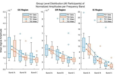
Figure 1: Group average LFO amplitudes for
baseline (T01) and endpoint (T03) for each frequency band in WM ROIs. Across
all ROIs and frequency bands a decreased in average amplitude was detected for
the low frequency neural oscillations.
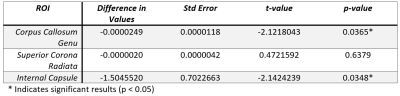
Table 1: Heteroskedastic linear mixed-effects
model ROI fixed effect results demonstrating significant decreased in LFO
average amplitudes between baseline and endpoint
-
Cerebrovascular Reactivity Mapping using Resting-State Functional MRI in Patients with gliomas
Mei-Yu Yeh1,2, Henry S Chen2, Ping Hou2, Vinodh A. Kumar3, Jason M Johnson3, Kyle R Noll4, Sujit S Prabhu5, Donald F. Schomer3, and Ho-Ling Liu 2
1Department of Biomedical Engineering and Environmental Sciences, National Tsing Hua University, Hsinchu, Taiwan, 2Department of Imaging Physics, The University of Texas MD Anderson Cancer Center, Houston, Houston, TX, United States, 3Departments of Diagnostic Radiology, The University of Texas MD Anderson Cancer Center, Houston, TX, United States, 4Department of Neuro-oncology, The University of Texas MD Anderson Cancer Center, Houston, TX, United States, 55Department of Neurosurgery, The University of Texas MD Anderson Cancer Center, Houston, TX, United States
1.rRS (regression RS)-CVR showed better agreement with BH-CVR.2.The optimal frequent bands for rRS calculation in glioma patients are consistent with previous studies 3.The agreements between rRS- and BH-CVR were better in normal tissue than in the lesion.
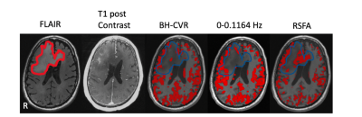
Fig.5 Imaging results from the one patient with gliomas. The first is lesion overlay on FLAIR image. The second one is T1 post contrast. The rest of all are spatial pattern among three CVR mapping approaches. The threshold of BH-CVR was set to 0.45. The threshold of rRS-CVR map was set to t>3.45(p<0.05). RSFA-CVR map was threshold such that the total activated fraction of gray matter in BH-CVR and RSFA map was equal.
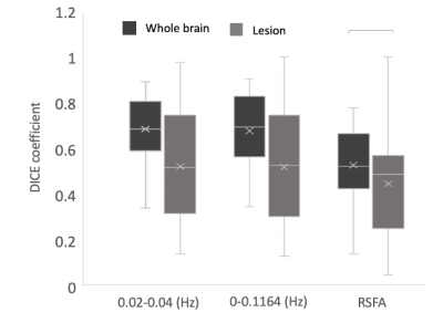
Fig.4 The dice coefficient between BH-CVR and three different methods of mapping CVR in normal brain tissue and in lesion (p<0.05).
-
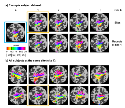
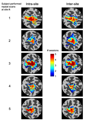
Long-term stability of cerebrovascular reactivity varies across brain regions
Stefano Moia1,2, Vicente Ferrer1,2, Rachael C Stickland3, Ross Davis Markello4, Eneko Uruñuela1,2, Maite Termenon1, César Caballero-Gaudes1, and Molly G Bright3,5
1Basque Center on Cognition, Brain and Language, Donostia, Spain, 2University of the Basque Country UPV/EHU, Donostia, Spain, 3Department of Physical Therapy and Human Movement Sciences, Feinberg School of Medicine, Northwestern University, Chicago, IL, United States, 4Montreal Neurological Institute, McGill University, Montreal, QC, Canada, 5Biomedical Engineering, McCormick School of Engineering and Applied Sciences, Northwestern University, Chicago, IL, United States
We found that long-term stability of cerebrovascular reactivity and its lag response presents regional patterns that can be explained equally by vascular anatomy, neural activity, and anatomical structures.
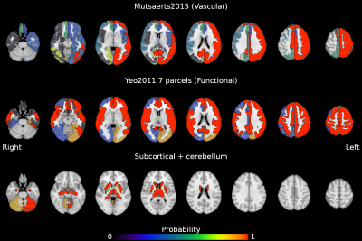
Figure 3: Probability map of the reliability of CVR being locally specific (i.e. homogeneous). Areas with a probability > 0.99 are delineated with a solid border. Volumes are in radiological space.

Figure 4: Probability map of the reliability of lag being locally specific (i.e. homogeneous). Areas with a probability > 0.99 are delineated with a solid border. Volumes are in radiological space.
-
Non-calibrated Equations for Quantification of Local fMRI Signal Changes with Hemodynamic Oxygen Metabolism (CBF and CMRO2)
Linqing Li1, Sean Marrett1, Andy John Derbyshire1, and Peter Bandettini 2
1Functional MRI Facility/NIMH, National Institutes of Health, Bethesda, MD, United States, 2National Institute of Mental Health, National Institutes of Health, Bethesda, MD, United States
We derived a simple coupling relationship for changes of CMRO2 calculation as (CMRO2/CMRO20)=(CBF/CBF0)0.25 when α=0.38, β=1.5. It is suggested that percentage changes of CMRO2, δ(CMRO2), can be directly calculated from changes of CBF without prior knowledge of M.
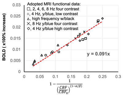
Figure. 3 Fitting results for M parameter determination based on graded visual stimulation data adapted from Fig. 7a of Hoge, et al., MRM, 1999. Data were acquired with 2, 4, 6 and 8 Hz stimulation under different contrast and colors. Based on our Eq. 5, linear fitting result of M was determined to be 0.09, which is approximately in line with M parameter in Davis work shown in Figure. 2. Note, this M=0.09 is significantly different from M=0.22 from its CO2 calibration approach, potentially due to instability of CO2 approach.
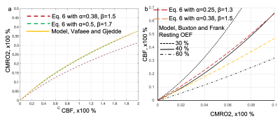
Figure. 4 Comparisons of Eq. 6 with oxygen delivery models. Fig. 4a, In model from Vafaee and Gjedde, curve green line was calculated with parameters of Ca, arterial oxygen concentration 7.8 mmoI/L, L the average oxygen diffusion capacity 4.09 μmol/hg-1min-1 per mm Hg-1), P50=26 mmHg and h, Hill coefficient of the oxygen dissociation curve, 2.84. Fig. 4b, in model from Buxton and Frank, three resting OEF values were simulated as 30%, 40% and 60% as the model is sensitive to the resting OEF. Eq. 6 curves red and yellow dash lines were calculated from different α and β values.
-
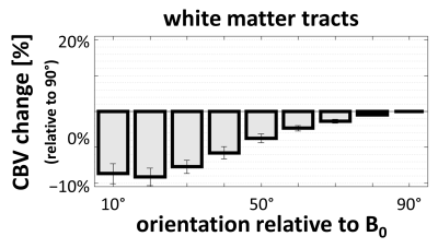
Modeling the vascular influences on BOLD fMRI using in vivo brain vasculature: incorporating vessel diameter, orientation, and susceptibility
Michael Bernier1,2, Jeorg Peter Pfannmoeller1,2, Saskia Bollmann3, Avery J.L. Berman1,2, and Jonathan R Polimeni1,2,4
1Department of Radiology, A. A. Martinos Center for Biomedical Imaging, Massachusetts General Hospital, Boston, MA, United States, 2Radiology, Harvard Medical School, Boston, MA, United States, 3Centre for Advanced Imaging, University of Queensland, Brisbane, Australia, 4Division of Health Sciences and Technology, Massachusetts Institute of Technology, Boston, MA, United States
We have developed
a “forward-model” method to calculate the extravascular fields surrounding the
blood vessels of the brain that accounts for the vessel diameter and
orientation and estimates the field change with activation using in vivo
measures of vessel anatomy and blood susceptibility.
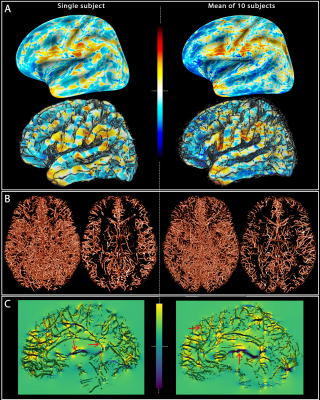
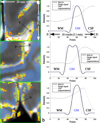
Fig. 1: Field offsets
surrounding major blood vessels The left panels illustrate the results for a single-subject while the right panels are the mean computed for all the subjects. (A) The field offset are projected on both inflated and GM surfaces obtained using Freesurfer. (B) The segmented vessels, illustrated in 3D and in a cross-section (20 mm), are overlapped on the delta B maps (C) to show the strong dipole effects surrounding the vessels perpendicular and parallel to B0 (red arrows).
-
Biophysical simulations of the BOLD fMRI signal using realistic imaging gradients: Understanding macrovascular contamination in Spin-Echo EPI
Avery JL Berman1,2, Avery JL Berman1,2, Fuyixue Wang1,3, Kawin Setsompop4,5, J. Jean Chen6,7, and Jonathan R Polimeni1,2,3
1Athinoula A. Martinos Center for Biomedical Imaging, Massachusetts General Hospital, Charlestown, MA, United States, 2Department of Radiology, Harvard Medical School, Boston, MA, United States, 3Harvard-MIT Division of Health Sciences and Technology, Massachusetts Institute of Technology, Cambridge, MA, United States, 4Department of Radiology, Stanford University, Palo Alto, CA, United States, 5Department of Electrical Engineering, Stanford University, Palo Alto, CA, United States, 6Rotman Research Institute, Baycrest Health Sciences, Toronto, ON, Canada, 7Department of Medical Biophysics, University of Toronto, Toronto, ON, Canada
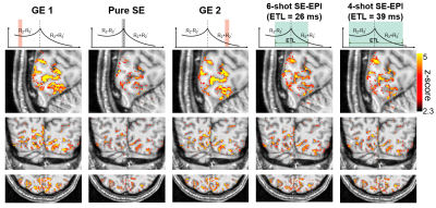
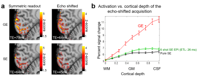
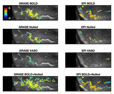
We introduced BOLD signal simulations that incorporate image encoding gradients. We examined large-vessel Spin-Echo BOLD contamination as a function of EPI readout duration, vessel size, voxel size, and cortical depth, and reproduced experimental results related to the readout duration.
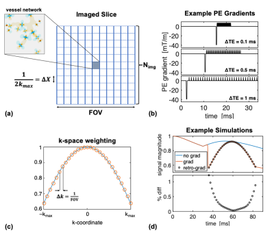
Fig 1: Schematic of the image-encoding framework. (a) Overview of the "imaged" slice, consisting of the simulated vessel network at its center and surrounded by zero magnetization, effectively a Kronecker delta-function. (b) Example EPI PE gradient train at multiple echo-spacings. (c) The sinc-weighting imposed by the encoding gradients. (d) Example SE simulations without imaging gradients (blue), with imaging gradients (orange), and with the k-space weighting retrospectively applied to the non-encoded simulation (black circles). The difference is up to a maximum of ~1%.
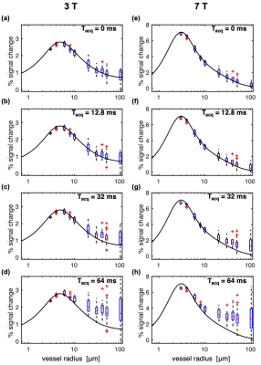
Fig. 3: Box plots of SE-BOLD percent signal change vs. vessel radius for multiple acquisition window durations (Tacq), and where the voxel size was held constant, resulting in decreasing numbers of vessels for the larger radii. Simulations were performed at 3T (left) and 7T (right) with Tacq increasing from 0 (a,e) to 64 ms (d,h). For comparison, the black curves are the spline fits to the SE data with Tacq = 0 ms in Fig. 2. Phase-encoding gradients were incorporated retrospectively as described by Eq. (2) in the Methods. Note the different scales for 3T and 7T.
-
Numerical simulations to investigate the contribution of arteries and veins to the relative BOLD-fMRI signal change by means of SO2 and CBV changes
Mario Gilberto Baez-Yanez1, Alex Bhogal1, Wouter Schellekens1, Jeroen C.W. Siero1,2, and Natalia Petridou1
1Department of Radiology, Center for Image Sciences, University Medical Center Utrecht, Utrecht, Netherlands, 2Spinoza Centre for Neuroimaging Amsterdam, Amsterdam, Netherlands
Gas challenges during BOLD-fMRI is appealing to study hemodynamic changes. With the support of computational
modeling, gas manipulations provide a means to infer vascular contributions. We
show look-up tables of the possible vascular contribution
responsible for measured BOLD signals
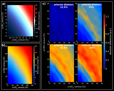
Look-up
tables obtained from a representative RVN model. (a)
shows the relative BOLD-fMRI signal change assuming SO2
changes for arteries and veins, separately, while CBV is kept constant (arterial basal SO2=98%;
venous basal SO2=60%).
(b) Look-up table for different SO2/CBV
changes in the venous compartment assuming an arterial basal-state
(arterial SO2=98%,
arterial dilation=0%). (c) show the absolute difference between the
basal-state (b) and different percentages of arterial dilation states
(12.5%, 25%, 37.5%, 50%) while the arterial SO2
is constant at 98%.
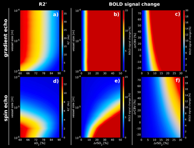
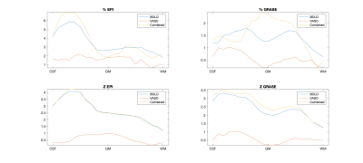
R2’
and relative BOLD-fMRI signal changes obtained from an artificial
vascular network for GE and SE at 7T assuming different SO2
and CBV changes. (a, d)R2’ calculated for different vessel sizes
–ranging from 1µm to 100µm- for GE(TE=27ms) and SE(TE=45ms).
(b, e)relative BOLD-fMRI signal change for different vessel sizes
and increments of SO2
levels for GE and SE. (c, f) relative BOLD-fMRI signal change
assuming CBV changes for GE and SE, respectively. GE shows a higher
sensitivity to small volume changes with respect to small SO2
changes in contrast to SE.
-
Simulating the BOLD fMRI transverse relaxation at 3 T: How accurate is the 2D approximation?
Jacob Chausse1, Avery J. L. Berman2, and J. Jean Chen1,3
1Rotman Research Institute, Baycrest Health Sciences, North York, ON, Canada, 2A. A. Martinos Center for Biomedical Imaging, Harvard Medical School, Massachusetts General Hospital, Boston, MA, United States, 3Department of Medical Biophysics, University of Toronto, Toronto, ON, Canada
2D and 3D Monte Carlo simulations of the transverse relaxation rate show excellent agreement. This finding establishes the validity of the 2D approximation as a faster, less memory-intensive alternative.
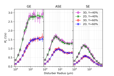
Figure 4. R2’ vs. Vessel Radius: comparing blood oxygenation with 2D MC and 3D MC for gradient echo (GE), asymmetric spin echo (ASE) and spin echo (SE). Uses CBV=2%, Hct=35.7%.
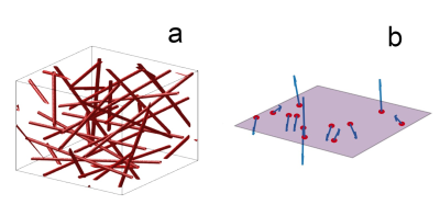
Figure 1. Visualization of the simulated voxels: (a) 3D voxel in a cube, where red cylinders represent blood vessels (b) 2D voxel on a plane where the vectors (blue) indicate the direction B0 at the vessel cross sections (red).